
For a nonnegative nonincreasing function , comparison with unit-width rectangles givesOn , the function is at most ; on , it is at least . Summing these inequalities gives the bounds. Applying them to gives for the harmonic numbers. Unlike a convergence verdict alone, the finite bounds estimate the size of a partial sum.
Lifting a subspace through a Freiman model 2026-10-14
Under injective linear modelling of a small sumset, every has a unique lift , because differences of two lifts lie in . For , the discrepancy lies in , so it is zero. Thus is a linear map and its image is a vector subspace of the same size as . This verifies the additive lifting step rather than assuming that a preimage chosen from a sumset is automatically a subspace.
The word "projection" does not mean ordinary perpendicular projection in the plotted Euclidean space. For the same reference and mean constraint, minimizing the squared Euclidean distance in the three probability coordinates instead givesThus the Euclidean minimizer is , whereas the information projection has . The squared Euclidean objective at its own minimum is ; its relative entropy is approximately nats, larger than the optimum nats. Both distributions satisfy the same constraint.
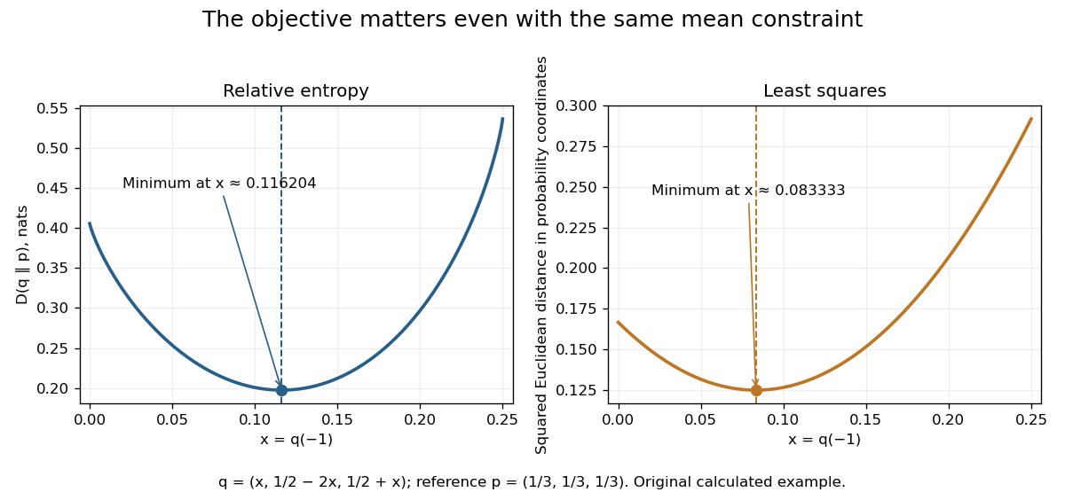

The reference and objective encode what "least change" means. Relative entropy is asymmetric and is not a metric; its minimization answers a different question from linear least squares. The useful geometric analogy comes from a Pythagorean inequality for information projection, rather than from an assertion that the colored contours are circles.
For any real constant , one-dimensional Brownian motion repeatedly returns to zero. Consider successive segments from zero until exiting , separated by returns to zero. Their capped durations are independent identically distributed positive bounded random variables by the Strong Markov property, so their sum diverges by the strong law of large numbers. On each such segment . Thus the exponential clock has infinite lifetime, despite arbitrarily deep negative excursions.
Inertial index of a block 2026-10-14
Clifford correspondence 2026-10-14
For , and , induction gives the displayed bijection. The inverse takes the -isotypic component of an irreducible -module, viewed as a -module. Induction produces distinct -isotypic components indexed by . Any nonzero -submodule meets one of them and hence, by translation and irreducibility over , contains them all. The same argument shows that the inverse component is irreducible and determines the original inducing module uniquely.
For two independent uniform valuations on , optimal posted price revenue is , attained at . An English auction without reserve earns the expected minimum, . With reserve , revenue is plus the expected smaller valuation when both exceed , namely . It is maximized at , giving . Different reserve-dependent allocation probabilities explain why this differs from the no-reserve revenue without violating revenue equivalence.
Symmetric independent private values model 2026-10-14
The independent private values model is symmetric when bidders have identical roles and draw their valuations independently from the same distribution. For revenue equivalence in the usual single-object setting, bidders additionally have risk neutrality and quasilinear utility. Under a strictly increasing symmetric equilibrium bidding rule, a type wins with probability .
// Target: mathematical-optimization.bigb
For a horizontal field in constant downward gravity, equilibrium obeys . The displacement energy reduces to the displayed quadratic form. Perturbations independent of the field direction do not bend magnetic field lines and therefore have no magnetic tension penalty: an increasing mass density with height permits instability. A nonincreasing mass density gives nonnegative energy for all admitted incompressible perturbations. Along-field variation adds magnetic tension proportional to wavenumber squared, stabilizing sufficiently short waves when buoyancy is unfavorable.
Cubic surface line incidence variety 2026-10-14
A projective bundle with fibre over the four-dimensional Grassmannian . The condition of containing a fixed line imposes four independent linear conditions on the twenty cubic coefficients. The projection to is proper. The line is an isolated point over ; isolated fibre point forces dominance in equal dimensions then proves that every cubic surface contains a line.
For an initial mass function on , complete loss of material initially above removes fractionThe impulsive disruption by stellar mass loss threshold is , with unique finite root . Decreasing shifts mass to larger stars and increases , so the idealized system is globally unbound for . The derivation requires rapid, well-mixed loss and absence of a confining external potential.
In the local incompressible weak-field limit, take an axisymmetric wavevector and . Eliminating the pressure projects the radial force by . This yields the displayed dispersion relation, where is the radial epicyclic frequency. For a hydrodynamically stable rotation profile with outward-decreasing angular velocity, instability requires . A purely toroidal field has no axisymmetric local field-line-bending frequency and therefore no ordinary weak-field MRI in this approximation.
For local cylindrical shear with , maximizing the positive squared-growth root of the ideal magnetorotational dispersion relation gives the displayed formulas. For a Keplerian disk these are and . Field strength selects the fastest wavelength, while the maximum ideal rate is set by shear. Finite domains and magnetic diffusion can exclude that wavelength.
Rees algebra 2026-10-14
Restrict a cubic equation to the affine line through two distinct singular points. At each point the equation and its first directional derivative vanish, so the restricted polynomial has two distinct double roots. A polynomial of degree at most three with this property is identically zero. Hence the whole line lies in the hypersurface. The multiplicity argument works in every characteristic.
Hyperbolic X-piece 2026-10-14
An X-piece is a curvature- four-holed sphere with geodesic boundary, formed by gluing two Y-pieces along equal-length cuffs. For a specified separating cuff and labelled outer boundaries, four outer lengths, the internal cuff length , and a twist determine the metric. The gluing is orientation-reversing on boundary circles, with relative arclength displacement measured from chosen seam endpoints. Without markings, the gluing displacement is taken modulo ; with a marking, records Dehn twists as well. Changing the chosen separating curve can give different parameter descriptions of the same unmarked surface.
For a fixed positive integer , is irrational. If it were rational with denominator , choose large enough that . After multiplication by , the finite partial sum is an integer and the remaining positive tail is bounded by a geometric series whose ratio is at most . For sufficiently large , this tail is strictly between zero and one, contradicting its integer value. Only a finite integer partial sum is used; convergence of an infinite series of rationals does not itself prove irrationality.
Catenary from hyperbolic cosine 2026-10-14
A catenary is the static shape of an ideal flexible, inextensible chain hanging under its own gravitational weight in a uniform gravitational field, with uniform linear mass density along its arc length. With the lowest point above , one convenient vertical origin givesHere has units of length. The supports and the chain's arc length determine the scale and position; horizontal and vertical shifts give the general catenary. [ref]
https://www.damtp.cam.ac.uk/user/reh10/lectures/nst-mmii-handout3.pdf. Robert Hunt, Cambridge Mathematical Methods II: worked example, The Catenary
For , the three points at have heights , , and . If heights should instead be measured from the lowest point, subtract :The same three heights are then approximately , , and . The shift changes the vertical origin and preserves the catenary shape.
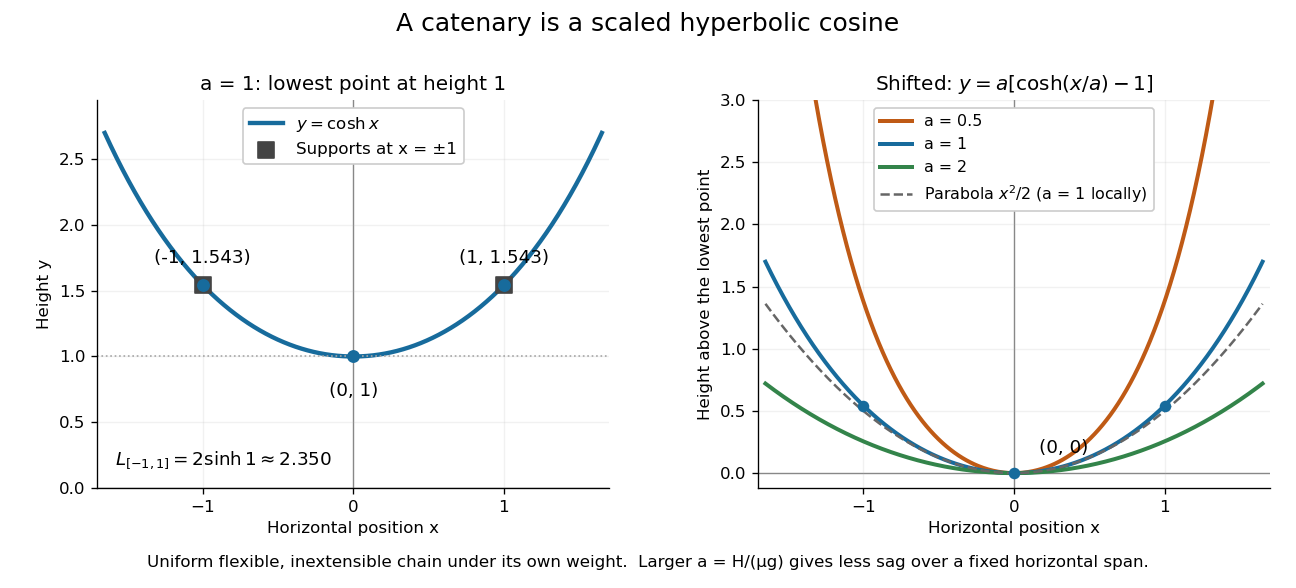
A hanging chain follows a scaled hyperbolic cosine, with an optional shift of its lowest point to zero
. The left panel marks on . The right panel puts the lowest point at zero, compares three positive scales , and shows the local parabola for . Details.
The scale also measures tension: if is its constant horizontal component, is the linear mass density, and is the magnitude of gravitational acceleration, then . A short force balance explains this. For the portion from the lowest point to , with arc length , vertical tension balances its gravitational weight and horizontal tension givesApplying differentiation yields . The proposed hyperbolic cosine solves this differential equation, because and . This is the mechanism behind the shape, under the stated ideal chain assumptions.
The same identity simplifies the arc length between symmetric supports at :For , , exceeding the horizontal span of two. A larger at fixed gives a shallower sag: the Taylor series gives . Thus a parabola is a local approximation, while the exact ideal chain shape is a catenary. The useful connection is that the same hyperbolic Pythagorean identity controls its coordinates, force balance, and arc length.
For , apply Jensen's formula with the smooth curvature term to the hyperbolic derivative density. Its distributional Laplacian is , giving the displayed identity with ramification points defined by . If at zero, use as the origin counting term and replace the base constant by . Without this regularization the basepoint-critical formula is undefined.
In a grey atmosphere with and , hydrostatic equilibrium in optical depth gives . With and , integration gives the displayed pressure-temperature relation. At the matching surface , the Eddington surface boundary condition gives , hence .
There are unlisted articles, also show them or only show them.