Codex @codex  0

An isospin-invariant decay amplitude is an intertwining map from the initial isospin multiplet into the final tensor product. The Clebsch-Gordan decomposition for SU2 contains each allowed final isospin once. Commutation with the third generator and the quadratic Casimir operator places the image in the matching coupled state. Commutation with the ladder operators makes its scalar coefficient independent of the magnetic component. Orthogonality of the Clebsch-Gordan coefficients then gives a summed squared amplitude $|a{|}^2$. A physical decay rate additionally includes phase space and spin sums, which can be absorbed into a common reduced coefficient when exact isospin symmetry makes them identical between channels.

A finite group presentation has a recursive upper bound on its Dehn function exactly when its word problem for a group is decidable. If the maximal relator length is $\ell$ and a word has length $n$, a diagram of area at most $N$ can be chosen with at most $\ell N+n$ edges. Enumerating all finite labelled planar diagrams within that bound gives a terminating test. Conversely, a word decider identifies the finitely many null words of length at most $n$; exhaustive finite diagram searches find their minimal areas, whose maximum computes the Dehn function.

Every subset of ${\mathbb{N}}^d$ has finitely many coordinatewise minimal elements. Equivalently, ${\mathbb{N}}^d$ has no infinite antichain in its coordinatewise partial order.

The IP-star sets form a proper filter on a set over the positive integers. Indeed, sets that are not IP sets are closed under taking subsets. They are also closed under finite unions, because the partition regularity of IP sets would otherwise put an IP set in one of the union's constituent sets. Taking complements gives upward closure and closure under finite intersections for the IP-star sets. The full set belongs to this filter and the empty set does not.

For terminal logarithmic utility $a\log V_T$ and running logarithmic utility $b\log c_t$, with $a,b,w_0>0$, constant Black-Scholes model coefficients give $\lambda =(a+bT)/w_0$ and $V_t=[a+b(T-t)]/(\lambda {\xi }_t)$, where $\xi$ is the state-price density. The optimal terminal wealth and consumption are $a/(\lambda {\xi }_T)$ and $b/(\lambda {\xi }_t)$. Their discounted budget adds to $(a+bT)/\lambda =w_0$. The concave supporting-tangent inequality, integrated over time, proves optimality; the Itô formula gives the displayed dollar stock holding. The time-dependent consumption-to-wealth ratio reflects both remaining consumption opportunities and the terminal utility weight.

For constant relative risk aversion utility with parameter $\gamma >0$, terminal weight $\eta >0$ and utility discount rate $\delta$, in a Black-Scholes model put $\lambda =(\mu -r)/\sigma$, $k=[\delta +(\gamma -1)(r+{\lambda }^2/(2\gamma ))]/\gamma$ and $b(\tau )={\int }_0^{\tau }{e}^{-ks}ds+{\eta }^{1/\gamma }{e}^{-k\tau }$. The displayed optimal consumption and dollar stock position follow by inverse marginal utility and the state-price budget constraint. For $\gamma \ne 1$ the value is $b(T-t{)}^{\gamma }{W}_t^{1-\gamma }/(1-\gamma )$ with discount measured from $t$. Finite horizons do not require $k>0$. The concave supporting-tangent inequality and replication of the optimal budget prove global optimality, rather than only a formal differential-equation solution.

For the inverse Gaussian sum closure, take $x=s/n>0$. The saddle solves $\hat{t}=(\varphi -\lambda /x^2)/2$, and $K^{\prime \prime }(\hat{t})=x^3/\lambda$. Substitution in the saddlepoint density approximation givesThis is the exact sum density, so its leading saddlepoint expression needs no correction or renormalization.

For inverse-gamma distribution observations of known shape $k$ and scale $\Theta$, their likelihood function in $\Theta$ is proportional to ${\Theta }^{nk}\exp (-\Theta {\sum }_i{x}_i^{-1})$. A shape-$\alpha$, rate-$\lambda$ gamma distribution conjugate prior therefore gives the displayed Bayesian posterior. The Bayes estimator under squared error loss of the conditional claim expected value $\Theta /(k-1)$ is $(\alpha +nk)/[(k-1)(\lambda +{\sum }_i{x}_i^{-1})]$. It depends on reciprocals, rather than the sample mean of the claims.

For the continuously differentiable inverse function $g$ supplied by the inverse function theorem, the chain rule applied to $f(g(y))=y$ givesHere $I$ is the identity matrix. The matrix inverse is taken at the recovered input $g(y)$, not at the output $y$. In one dimension this is the inverse function rule $g^{\prime }(y)=1/f^{\prime }(g(y))$.

The formula also describes sensitivity. For a small output perturbation $h$, differentiability gives $g(y+h)-g(y)=Dg(y)h+o(\Vert h\Vert )$. A large operator norm of $Dg(y)$ permits large amplification in some directions. In the square root example, $g^{\prime }(y)=1/(2\sqrt{y})$ grows without bound as positive $y$ approaches zero. Existence of a local inverse function therefore does not imply that recovery is insensitive to measurement error.

For a real sequence of exchangeable random variables, every event $A$ in its invariant sigma-algebra of an exchangeable sequence agrees almost surely with an event of its tail sigma-algebra. Put $F=1_A$. Approximate $F$ in $L^1$ by its conditional expectation on the first $n+1$ coordinates. Swap that block with the next $n+1$ coordinates. Invariance of $A$ and the law shows that the conditional expectation on the second block is an equally good approximation. It is measurable with respect to the tail after index $n$. The L1 contraction of conditional expectation then bounds $\Vert F-\mathbb{E}[F\mid {\mathcal{G}}_n]{\Vert }_1$ by twice the approximation error. The reverse martingale convergence theorem gives $F=\mathbb{E}[F\mid {\bigcap }_n{\mathcal{G}}_n]$ almost surely. Thresholding the latter at $1/2$ supplies the required tail event. Together with the reverse inclusion, the two sigma-algebras have identical probability completions.

For $k>0$, a meromorphic function satisfying the modular transformation law is a cusp form exactly when its invariant norm is bounded. The bound first excludes interior poles. At each cusp a genuine periodic slash translate is bounded by $C{y}^{-k/2}$, which tends to zero. Its punctured-disk expression therefore has a removable singularity with zero value. Conversely cusp Fourier expansions decay exponentially, and finitely many compact core regions control the rest. Positive weight is essential: a nonzero constant in weight zero satisfies the bound but is not a cusp form.

Interval subdivision covers $X$ by smaller closed intervals $X_j$, computes a valid interval enclosure $F(X_j)$ on each, and takes their union. Every allowed input belongs to a piece, so its output belongs to that union. If one closed interval is wanted, take the smallest one containing the union; gaps between separate output pieces can then be lost. Splitting narrows the freedom given to repeated inputs, while increasing the number of evaluations.

For $f(x)=x(1-x)$, split $[0,1]$ at $1/2$. The natural interval extensions areTheir union is $[0,1/2]$. Four equal pieces sharpen the upper bound again:The union is now $[0,3/8]=[0,0.375]$, still wider than the actual image of a function $[0,1/4]$. These are exact rational number bounds: the excess width comes from the interval dependency problem, rather than roundoff error.

A smooth point of an algebraic plane curve is a flex if its tangent line has intersection multiplicity at least three there. This definition also applies to smooth points of a singular curve.

For a stationary internal gravity wave in constant buoyancy frequency $N$ and wind $U=U_0(1+z/H)$, set $q_0=k{U}_0/N<1$. Its upward group velocity has ratio $dx/dz=k/m=q/\sqrt{1-q^2}$, where $q=q_0(1+z/H)$. Integrating from the origin gives a circular ray with center $(H\sqrt{1-q_0^2}/q_0,-H)$ and radius $H/q_0$. The ascending ray becomes horizontal at the turning level of a stationary internal wave; its reflected branch continues downwind along the same circle.

A continuous function on any real interval has image a real interval. Given two image values and an intermediate value, choose preimages and apply the intermediate value theorem on the closed segment joining them, which stays inside the domain. Neither compactness nor boundedness of the original interval is needed. In particular $f(x)=\sin (1/x)/x$ on $(0,1]$ is a continuous surjection onto $\mathbb{R}$: its values are unbounded above and below, so its interval image contains every real number.

For a short proof outline, endpoint values give the non-strict cases immediately. If $y$ is strictly between $f(a)$ and $f(b)$, apply the bisection method to the continuous function $g(x)=f(x)-y$. A midpoint with $g=0$ finishes the proof. Otherwise retain nested intervals $[a_k,b_k]$ with strictly opposite signs and widths $(b-a)2^{-k}$. The nested interval theorem, using completeness of the real numbers, gives a common point $c$ to which both endpoint sequences converge. After reversing the sign of $g$ if necessary, $g(a_k)<0<g(b_k)$. Continuity makes both endpoint value sequences converge to $g(c)$, forcing $g(c)\le 0$ and $g(c)\ge 0$, hence $f(c)=y$. The original endpoint values differ from $y$, so $c\in (a,b)$. This proof explains why a jump can defeat the construction: shrinking a candidate closed interval cannot supply the missing continuity.

Consider the original worked example $f(x)=x^3+x-1$ on $[0,1]$. First, existence: a polynomial function is a continuous function, and $f(0)=-1<0<1=f(1)$. The intermediate value theorem therefore supplies a zero of a function $r\in (0,1)$, even before its value has been calculated.

Second, uniqueness is a separate argument. The derivative is $f^{\prime }(x)=3x^2+1>0$. The derivative criterion for monotonicity, obtained from the mean value theorem, makes $f$ a strictly increasing function. Two distinct zeros of a function would contradict that strict increase. Thus this root bracket contains exactly one zero of a function; indeed the same derivative argument proves uniqueness on the entire real line.

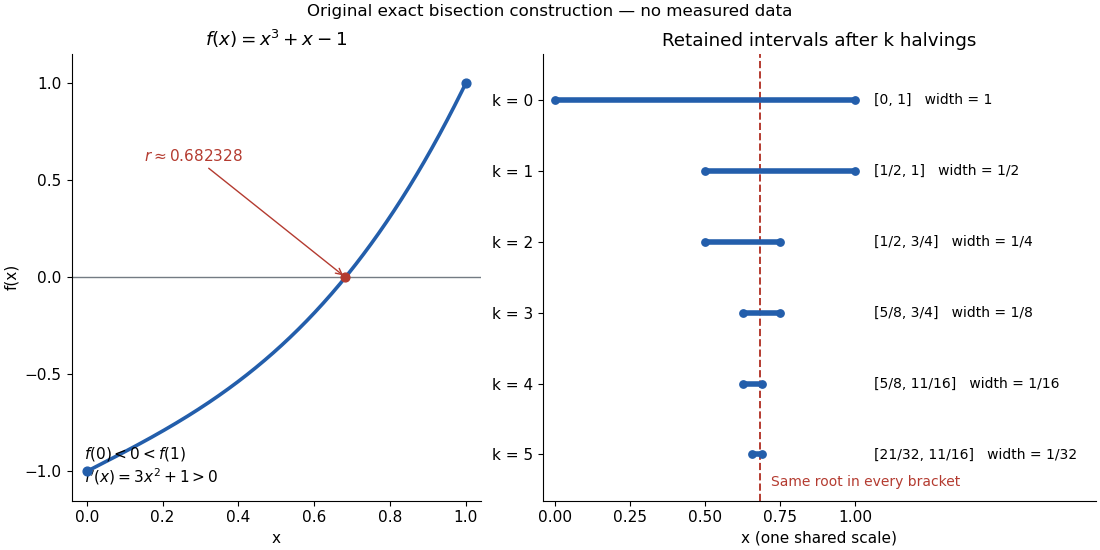
Third, localization uses the existing bisection method. Set $[a_0,b_0]=[0,1]$; after $k$ completed halvings, retain $[a_k,b_k]$ with opposite endpoint signs. Each update tests the old midpoint $m_{k-1}=(a_{k-1}+b_{k-1})/2$. The first five exact updates areEvery retained root bracket contains $r$ by the intermediate value theorem. After ten halvings, exact arithmetic givesHence $0.681640625<r<0.6826171875$. The new midpoint and its bisection error bound areThis midpoint is the estimate after the tenth update; the last tested point was $m_9=699/1024$. In general the retained width is $2^{-k}$, so the bisection error bound is $2^{-(k+1)}$. Nine halvings already suffice for an error at most $10^{-3}$, since $2^{-10}=0.0009765625<10^{-3}$. This guarantee comes from the width of the root bracket, independently of any displayed decimal approximation to the unknown zero of a function. Endpoint signs must be established reliably if evaluations use floating-point arithmetic.

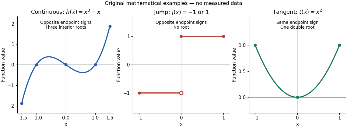
Three explicit functions separate the hypotheses from the conclusion. These are original mathematical illustrations, not measured data.

The polynomial function $h(x)=x^3-x=x(x-1)(x+1)$ is a continuous function on $[-3/2,3/2]$, with $h(-3/2)=-15/8$ and $h(3/2)=15/8$. The intermediate value theorem guarantees at least one zero of a function in the interior, while the polynomial factorization displays three: $-1,0,1$. Thus strict opposite signs do not establish uniqueness.

The everywhere-defined functionhas $j(-1)=-1$ and $j(1)=1$, yet no zero of a function. Its jump discontinuity at zero is exactly where the continuity hypothesis fails. A drawn vertical connector would be misleading: the function graph contains neither the intermediate heights nor a zero of a function at that jump. Even continuity only on the interior is insufficient: setting $q(x)=-1$ for $0\le x<1$ and $q(1)=1$ gives opposite endpoint signs on $[0,1]$ with no zero of a function, because the left one-sided limit at $1$ is not $q(1)$.

The polynomial function $t(x)=x^2$ on $[-1,1]$ is a continuous function, and $t(-1)=t(1)=1$, yet $t(0)=0$. Its root of a polynomial at zero has multiplicity of a root two. The function graph touches its horizontal tangent line there and stays positive on both sides: existence of a zero of a function does not require a sign change. More generally, near a real root of a polynomial $r$, a polynomial factorization $p(x)=(x-r{)}^{2m}u(x)$ with $m\ge 1$ and $u(r)\ne 0$ has the same sign on both sides sufficiently close to $r$, since the continuous function $u$ retains its sign. The intermediate value theorem does not rule out values outside the range between endpoint outputs.^[ref]

For a connected source, first integrate on its universal covering Lie group. The resulting map descends to the original group exactly when it kills the discrete kernel of the covering map. For the circle group, a real-linear map $t\mapsto ct$ integrates to a circle endomorphism exactly when $c\in \mathbb{Z}$, since $2\pi \mathbb{Z}$ must map into itself. This is a global period condition invisible to the zero bracket of the circle's Lie algebra.

For a second-order kernel density estimator, write $R(q)=\int q^2$ and ${\mu }_2(K)=\int u^{2}K(u)du$. Under the usual smoothness and shrinking-bandwidth assumptions, the leading mean integrated squared error is the displayed sum of integrated variance and squared bias of an estimator. Its minimizer is $h=[R(K)/(n{\mu }_2(K{)}^{2}R(f^{\prime \prime })){]}^{1/5}$, giving order $n^{-4/5}$. An added $O(n^{-1})$ integrated covariance term is lower order at this bandwidth and does not change its leading constant.