Derivatives can transfer risk, improve price discovery and permit hedging, so their existence is not by itself evidence that they cause crashes. They can also amplify stress through leverage, margin calls, counterparty exposure and forced dynamic hedging into falling markets. A short-gamma hedge can require selling more underlying after a fall, reinforcing feedback when liquidity is thin. The causal issue is the combination of positions, funding, market depth and institutional rules; derivatives are neither necessary nor sufficient for a crash, and correlation between trading volume and a crash does not establish the direction of causation.
The series is predictable in a statistical sense beyond linear return autocorrelation. For example, the observed past feature satisfies and , so its least-squares predictor within the family is . This is a predictor based on observed increments, not an assumption that the hidden driving signs are directly visible; it need not equal the full conditional expectation.
A finite bound on ordinary peak-to-trough financial drawdown does not follow. Choose a long alternating sequence of driving signs, . It produces , alternating and . The price never recovers during that episode and its cumulative loss grows without bound as the episode length grows. Every finite such driving sequence has positive probability. Thus
More precisely, over an -month window and over admissible starting histories, the maximum possible drawdown is
One derivation keeps the last two signs as a four-state dynamic program. Let be the smallest cumulative increment after steps ending with signs , with for each permitted initial pair. Then . Induction gives the negative of the displayed minimum. The bound is attained by increments for , or for , so it is also an attained peak-to-trough loss over months, not only an algebraic net displacement bound.
For comparison, the index with increments has , attained by successive negative signs; it too has no finite horizon-free bound. If “drawdown” were intended to mean a strictly decreasing consecutive run, the first model permits at most two successive increments, for a loss of four over two months, whereas the simple walk permits arbitrarily long such runs. That different run statistic must not be substituted for the usual drawdown definition: zero increments can separate continuing losses without any recovery.

Independent identically distributed increments have the same marginal distribution at every step and factorizing joint distributions across steps. With finite mean and variance , an additive random walk has mean displacement and variance after steps. Zero increment autocovariances follow from independence, but their converse is false. Gaussian increments are an additional assumption, not part of the definition of a random walk.
To investigate a measured price process, first specify the sampling interval and whether the model concerns price differences or log returns. Remove an estimated drift and examine stationarity, increment distributions, autocorrelations and variance growth over nonoverlapping horizons. Also test higher-order statistics, absolute or squared-return correlations, conditional distributions and out-of-sample predictability; those can reveal dependence missed by linear autocorrelation. Check whether different time scales and market regimes give compatible results, and account for bid-ask effects and intraday seasonality at short lags. Finite data cannot prove independence or permanent stationarity. Failure to reject a particular test is weaker than establishing that every joint distribution factorizes; the next example makes that distinction explicit.
Implied volatility is the volatility parameter that makes a specified option-pricing model reproduce an observed option price. For a call, it solves
For positive time to expiry and positive asset and strike prices, the Black-Scholes call price increases with , so an interior arbitrage-consistent price gives a unique finite positive value. It is an inverse model parameter, not the sample standard deviation of past returns or a guaranteed forecast of future realised volatility. Different implied volatilities across strikes or maturities form smiles or surfaces, signalling that one constant volatility does not fit all prices simultaneously.
Assume a non-dividend-paying tradable asset follows geometric Brownian motion , with constant volatility and risk-free rate . Trading is continuous, frictionless and divisible; borrowing and lending occur at the same rate, short selling is allowed, the strategy is self-financing, and there are no jumps or arbitrage opportunities. These are modelling assumptions, not assertions that market returns are exactly Gaussian or that hedging is costless in practice.
For a smooth option price , Itô's formula gives
Replicate it by shares and a cash account of value . Self-financing requires . Matching the stochastic term fixes . Matching the remaining drift and cancelling the physical drift then gives
This is the Black-Scholes equation. The cancellation does not assert that the actual expected asset return equals ; risk-neutral valuation is a consequence of replication under these assumptions.
For a European call, impose , with and for large . Its writer hedges the short option by holding shares and investing or borrowing the residual cash , rebalancing as and time change. In the constant-parameter model , where and is the standard normal cumulative distribution. Continuous rebalancing is an ideal limit: transaction costs, discrete trading, jumps and changing volatility create residual hedge risk. Writing the self-financing gains equation explicitly avoids incorrectly adding an unfinanced term to the strategy.
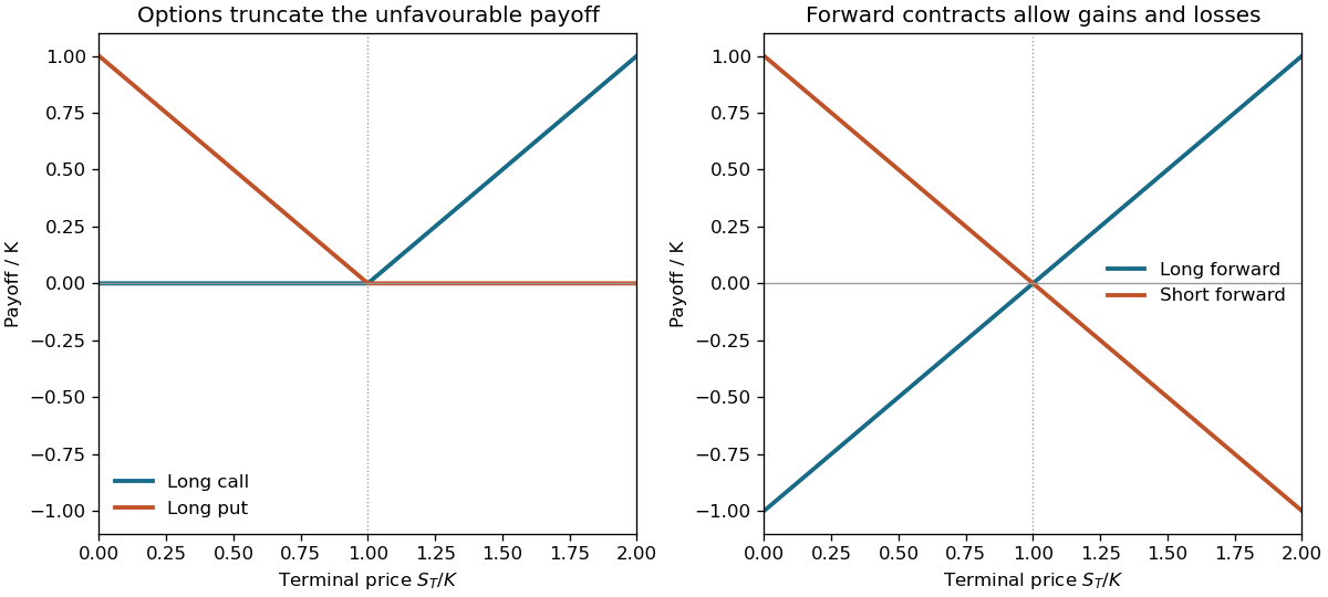
Let be the terminal asset price and a common strike or forward delivery price. A long European call and put have expiry payoffs
The call is zero below and then rises with slope one; the put falls with slope minus one below and is zero above it. A long forward instead has and a short forward has . Both are straight lines crossing zero at , with negative as well as positive outcomes.
The option's exercise right truncates the unfavourable side, whereas the forward is an obligation. These are payoffs, not total profits: an option premium and its financing cost have not been subtracted. A newly agreed fair forward may have zero initial value while still having a nonzero future delivery price.
Figure 1.
Original European call and put payoffs compared with long and short forward-contract payoffs
. Details.
Stylized facts of financial returns are robust qualitative statistical regularities found across many instruments or datasets, abstracting from their individual details. Examples include heavy return-distribution tails relative to a Gaussian model, weak linear autocorrelation of many liquid-market returns beyond short lags, and persistent clustering of large absolute or squared returns. Some markets also show asymmetric return-volatility responses and partial movement toward a Gaussian aggregate distribution at longer horizons.
These are empirical tendencies with sampling-scale and market qualifications, not exact universal equations. In particular, weak return autocorrelation does not imply independent increments: volatility clustering and higher-order dependence can remain. A useful model should state which regularities it explains and which its assumptions exclude, rather than treating one convenient random-walk model as an observed law.
For translation in a fixed direction , take and the preceding . The triple-product identity gives . Thus
Choosing the three Cartesian directions gives the three constants
These are magnetic pseudomomentum components, not the three components of kinetic momentum . A direct check is . In the stated gauge, , consistent with the Noether boundary correction.
Repeat the expansion in the strict-invariance proof, but now use . Along Euler-Lagrange trajectories,
It follows that the conserved Noether quantity is
The minus sign matters. It subtracts the boundary term created by the symmetry transformation. More explicitly, before using the equations of motion one has
The final sum vanishes on shell, proving the result for arbitrary coordinate-dependent under the source's fixed-time assumptions. It is this boundary-term form, rather than the uncorrected canonical momentum alone, that applies to translations in the magnetic example.
The canonical momentum for the stated symmetric-gauge Lagrangian is
Since is uniform and time independent, its Euler-Lagrange equation becomes
This is the magnetic Lorentz force, which is unchanged by constant spatial translations. The Lagrangian itself changes by
A total time derivative changes the action only by . For variations with fixed endpoints this boundary contribution has zero variation, so the equations of motion are unchanged. The translation is therefore a symmetry of the dynamics even though this particular gauge makes the Lagrangian only quasi-invariant.
Let and consider the infinitesimal fixed-time transformation . It induces . Expanding the Lagrangian gives
On a solution of the Euler-Lagrange equations, , so this equals . Exact invariance makes the left side zero, proving the fixed-time form of Noether's theorem:
The symmetry direction need not coincide with one original coordinate axis; can depend on the generalized coordinates. The conclusion is evaluated on physical trajectories, while the assumed invariance is a property of the Lagrangian under the transformation.
The Jacobi identity and the two brackets imply
Thus without re-solving the motion. Explicitly . Squaring and adding the two rotated components gives
Consequently the four quantities are not functionally independent: generically there are three independent constants. One may choose, locally, and the orientation encoded by ; their magnitude is fixed by the displayed relation. This also matches the maximum of three independent trajectory-labeling constants for a nonstationary autonomous flow in four-dimensional phase space. On singular subsets the local functional rank can be lower: for example, at and , the differentials of are proportional to , leaving at most two independent differentials together with ; “three” is the generic count, not an assertion about every singular configuration.
Put . The Hamiltonian has no explicit time or azimuthal dependence, so and . Its equations of motion are
Write . Differentiating along these equations gives
Equivalently, the same cancellation evaluates . Hence The extra conserved component is associated with the Runge-Lenz symmetry of this inverse-distance central potential, rather than with conservation of radial momentum.
Hamilton's equations are and . Using the elementary brackets from the previous part gives
A constant of motion is a function that stays unchanged along each physical trajectory. For a function with no explicit time dependence, the chain rule and Hamilton's equations give
Thus on the accessible phase-space domain. If a function explicitly depends on time, the criterion is instead ; the simpler statement uses the source's time-independent assumption.
For the canonical Poisson bracket, direct substitution of and gives
Therefore
This expresses the bracket as a first-order derivative acting on , with coefficients determined by ; it is the phase-space chain-rule form of the definition.
It can describe the motion per unit mass of a charged particle in the azimuthal magnetic field of a long straight current-carrying wire. Choose magnetic vector potential
Then and is the given Lagrangian. In terms of a straight-wire current , , so with signs fixed by charge and current direction.
A static magnetic force does no work, consistent with the conserved kinetic energy. Its radial component is and its axial component is , reproducing the radial and axial couplings above. The reference length in the logarithm is a gauge convention, not a new physical wire radius in the ideal exterior-field model.
Write , requiring and . The initial conditions fix and . At , the radial force is . Thus the unperturbed motion is the helix
To analyse a small initial radial velocity, eliminate the cyclic velocities using the conserved quantities. The radial energy equation is , with
Here and . The circular cylindrical radius is therefore stable. For , the first-order equation is , so
The orbit acquires small radial oscillations. The other coordinates are modulated consistently with the same constants:
These expressions retain the stated initial angular and axial velocities. The perturbation adds to the conserved energy. The expansion assumes , which follows from the supplied smallness condition when ; it is not an exact finite-amplitude helix.
The Euler-Lagrange equations in cylindrical coordinates are
The last two follow because and are cyclic coordinates. They give the conserved quantities
Since the Lagrangian is autonomous, its energy function is conserved as well:
The velocity-linear term cancels from this energy, but it still changes the equations of motion. A dimensionless logarithm means for some fixed reference length; replacing the printed by that expression changes the Lagrangian only by a total time derivative and shifts the numerical value of , not the trajectory.
Hamilton's principle states that the physical path makes the action stationary under differentiable variations vanishing at the fixed endpoints. Its conventional “least action” name does not guarantee a minimum. Expanding to first order and integrating the velocity term by parts gives
The endpoint term vanishes. By the fundamental lemma of the calculus of variations, the coefficients of the independent interior variations must vanish, yielding
For example, the zero path of a harmonic oscillator with endpoints zero can have both positive and negative second variations when the elapsed time exceeds a half-period; stationary action then need not be a least value. The Euler-Lagrange condition is the local statement that the variational principle actually supplies.
A plug-in hybrid electric vehicle can move short journeys to electricity while retaining liquid-fuel range for longer ones. It can reduce oil dependence and some local tailpipe emissions, but the carbon benefit depends on charging, trip length, electricity supply, vehicle manufacture and the fuel used when the engine runs.
For illustration, electricity consumption at grid intensity gives in use. A petrol vehicle using litres per km emits about from combustion under the paper's octane-density assumptions. Ignoring other life-cycle differences, their use-phase break-even electricity intensity is therefore roughly . Cleaner electricity improves the electric case; sufficiently carbon-intensive electricity can reverse it. These are conditional comparisons, not measured fleet averages.
A plug-in hybrid that is rarely charged may obtain little benefit while carrying both propulsion systems. Battery and fuel production also belong in a life-cycle assessment. Fully electric vehicles, efficient conventional vehicles, public transport, walking, cycling and reduced travel demand provide alternative or complementary routes. Plug-in hybrids can be a useful transition technology, but no physical argument makes them an essential component of every successful climate strategy.

There are unlisted articles, also show them or only show them.