Let be annual emissions abatement in tonnes per year. The given marginal abatement cost is
Under the stipulated global, stationary, unconstrained cost-benefit model, the optimal interior abatement equates that marginal cost to the avoided marginal damage of approximately per tonne. Thus
Total mitigation expenditure is the area under the marginal-cost curve, not its endpoint value times all abated tonnes:
The result also presumes baseline emissions permit this much reduction. Rational policy need not reproduce it: different discounting, damage uncertainty and risk aversion, income weights, omitted ecosystem impacts, adaptation and local air-quality benefits alter valued benefits; technology learning and adjustment constraints alter costs. Separate rational governments may abate less because some benefits accrue abroad, while cooperative policy can internalize those benefits. Future climate or technology changes also undermine a fixed present marginal-damage curve. These are changes in the optimization problem, not evidence of irrational decision-makers.
Insert the pulse response into and write . For a positive discount rate ,
Therefore
With , and the supplied one-tonne normalization of ,
This is valued at the time of emission because the discount factor is relative to that date. Valuing an emission at a future date from an earlier reference date would require an additional discount factor. The infinite-horizon integral converges for under the assumed persistent forcing.
For logarithmic forcing , where denotes atmospheric carbon-dioxide concentration rather than heat capacity, . Approximately constant in therefore requires a roughly constant conversion from emissions to persistent atmospheric burden and a concentration range small enough to hold fixed. Carbon removal must be negligible on the modeled horizon, or be replaced by a fixed retained fraction; a realistic multiscale carbon-cycle response generally violates the permanent-step approximation.
A one-tonne pulse at time is in tonne-normalized units. It gives a persistent forcing step . Convolving that step with the thermal response yields
There is no instantaneous temperature jump for finite , although forcing jumps. Both persistence and constant coefficients are deliberate simplifications, rather than an assertion that all emitted carbon dioxide remains airborne forever.
Put and assume , . The linear differential equation for a constant forcing step is
Multiplying by the integrating factor and integrating from zero to gives
The response initially grows at rate and tends to the equilibrium warming . Heat capacity per unit area and radiative-feedback units make an inverse time.
The quadratic coefficient must have units ; the printed makes its term dimensionally incompatible with a radiative flux. Interpret its numerical value as , with . The total imbalance is
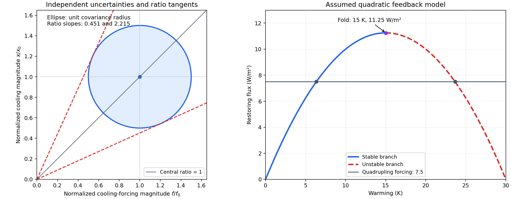
A quadrupling gives . The two equilibrium roots are
For positive heat capacity, stability requires . Thus only the lower root is stable. A saddle-node bifurcation occurs at
The logarithmic forcing relation gives . Strict linear stability holds below this concentration on the lower branch; the equality is marginal and is the supremum, not another strictly stable equilibrium. Sustained forcing above it causes warming without a balancing equilibrium in this quadratic model. At such large changes its local feedback expansion can fail, and other physics can intervene; it does not prove unlimited real-planet warming or locate a measured Earth runaway threshold.
Take the logarithmic forcing law with its normalization fixed by the given doubling value. Let be the positive magnitude of cooling and the positive magnitude of the earlier negative forcing:
At , . Equilibrium then yields
The concentration endpoints and imply forcing magnitudes and , approximately . Define normalized variables and . Independent approximately Gaussian uncertainties give the one-standard-deviation covariance ellipse
Its centre is and its principal directions are the two coordinate axes. Warming is , so rays from the origin have constant inferred warming. The bounding rays tangent to this ellipse have slopes satisfying , or
This gives the useful asymmetric one-parameter profile estimate
The concentration data supply only marginal intervals, not a full likelihood. This result explicitly approximates their logarithmic forcing uncertainty as Gaussian. Linear error propagation would instead give fractional uncertainty , or roughly , and misses the large reciprocal asymmetry. A unit-radius two-dimensional covariance ellipse itself contains about of a bivariate Gaussian, not ; the quoted interval uses the one-parameter profile/ratio construction, rather than claiming that ellipse is a joint region.
Figure 1.
Climate sensitivity from uncertain forcing and a quadratic feedback fold
. Original model plots: the left panel shows the normalized independent-uncertainty ellipse and tangent constant-sensitivity rays. The right panel plots the assumed quadratic restoring flux, its stable and unstable branches, and the finite forcing at which those equilibria merge. The fold is a property of this toy model, not an observed carbon-dioxide threshold. Details.
Use a positive stabilizing feedback coefficient: the net flux is . The Planck feedback increases outgoing thermal radiation as temperature rises and therefore contributes positively to . Water-vapor feedback raises infrared opacity as a warmer atmosphere holds more water, tending to reduce ; ice-albedo feedback also tends to reduce it as bright ice is lost. These signs depend on the explicitly stated convention.
For doubled carbon dioxide forcing , equilibrium gives
A symmetric positive interval maps to
The upward excursion is larger than the downward one because inversion is nonlinear. If the interval reaches zero, it supplies no finite upper bound on equilibrium warming within this linear stable model.
The actual Earth response to doubling carbon dioxide is expected to be much smaller than this roughly all-grey-absorbers estimate. Carbon dioxide absorbs in selected spectral bands rather than doubling opacity across the entire thermal spectrum, and doubling it does not double the other infrared absorbers. Saturated band centres and overlap with water absorption further distinguish it from uniform opacity multiplication. Changes in water vapour, clouds and the lapse rate introduce important climate feedbacks, but do not justify treating the real atmosphere as the stipulated dry, wavelength-independent absorber. The idealized number is therefore not an estimate of real-world equilibrium climate sensitivity.
Let be the mass mixing ratio of the uniformly mixed infrared absorbers, and let be their constant mass absorption coefficient. Hydrostatic integration gives downward optical depth . The useful fixed-tropopause-optical-depth approximation requires a sufficiently optically thick lower column, unchanged absorbed sunlight and upper radiative profile in optical-depth coordinates, and the same convective lapse law after the perturbation. Then the matching to the radiative region occurs at the same and temperature . Doubling all those absorbers gives
Assume also that the surface pressure is unchanged. A dry adiabat satisfies with . Consequently
for an initial Earth-like surface temperature . Its first-order logarithmic estimate, , is about ; the finite-doubling formula is preferable because the perturbation is large. This estimate is conditional on fixed and dry convective adjustment, not on carbon dioxide's measured spectral behavior.
There is also a consistency limitation to the most literal opacity model. A self-contained plane-parallel grey atmosphere with constant mass opacity has and . Its radiative logarithmic gradient is
It is therefore subadiabatic for these dry heat capacities, so it does not by itself establish the assumed deep dry convective column. The preceding warming is the intended fixed-matching-level, convectively prescribed estimate. A fully self-consistent model needs opacity varying with pressure, other heating structure or another closure to supply that convection; the two statements should not be silently identified.
Assume a well-mixed ideal gas with constant , no latent heat, and sufficiently strong surface heating to maintain dry convection near the surface. An adiabatically displaced unit mass has specific volume , so the stated relation and hydrostatic equilibrium give
This is the dry neutral lapse rate; infrared absorption alone does not guarantee that a radiative profile is steep enough to trigger convection. Combining the same equations with the ideal gas law yields along that adiabat.
High above the main infrared-emitting region, optical depth to space becomes small. A transparent-to-sunlight atmosphere has no substantial direct solar heating there; a thin grey layer absorbs the upwelling planetary infrared flux and emits from both faces. In the optically thin radiative-equilibrium limit,
The factor four in is projected-area versus whole-sphere averaging; the additional factor two counts emission upward and downward by the tenuous layer. For Earth-like and , this is about . Thus temperature approaches a height-independent skin value as , rather than continuing the dry adiabat to zero. This is an asymptotic grey-atmosphere approximation, not a proof that an entire finite stratosphere is exactly isothermal.
The tropopause is the transition between the lower, often convecting troposphere and the more stably stratified atmosphere above, where the decrease of temperature with altitude weakens or reverses. Its definition concerns the thermal profile, not a fixed universal altitude. An optical depth is a dimensionless path-integrated extinction, for mass extinction coefficient ; without emission into the ray its direct intensity is attenuated by .
In hydrostatic equilibrium, the upward pressure force balances weight:
The second equality uses the ideal gas law with specific gas constant . For constant and ,
For variable temperature the corresponding result is . The fixed-temperature derivative does not require the entire column to be isothermal.
Nonbaryonic dark matter can provide the additional gravitating mass. Gravitational lensing independently maps cluster mass, while the cosmic microwave background and Big Bang nucleosynthesis constrain the cosmic matter and baryon budgets. The separation of lensing mass from strongly interacting X-ray gas in merging clusters is evidence that much of the gravitating component is not that hot gas.
Uncounted baryonic matter, including the observed hot gas, faint stars and compact remnants, certainly adds to the stellar estimate. X-ray emission directly establishes a large gas reservoir. However, baryon-budget constraints and microlensing constraints on compact objects prevent arbitrarily filling the entire discrepancy with ordinary hidden objects.
Modified gravity could change the inference from a measured acceleration to a Newtonian mass. Such a theory must also reproduce the observed lensing and cosmological evidence; explaining some rotation curves alone is insufficient, and cluster mass discrepancies remain a demanding test. Departures from equilibrium and projection can bias individual mass estimates, but would have to explain the independent observations systematically rather than merely modify one virial prefactor.
For an isotropic velocity dispersion, . To specify the order-unity structure factor, approximate the gravitating system by a uniform sphere, whose gravitational potential energy is . The virial theorem gives
The numerical value uses and . Different mass profiles change the prefactor, rather than the scaling .
For fully ionized intracluster gas, take mean particle mass with . In the same uniform-sphere virial estimate, replace by to obtain
Alternatively, hydrostatic equilibrium gives . An isothermal gas with density proportional to gives . The supplied radius and temperature do not specify the profile, so the meaningful inference is a mass of order , with the displayed model choices making the coefficient explicit. The high supplied temperature need not yield the same estimate as the galaxy dispersion in a crude single-profile calculation.
The stellar estimate is much smaller:
It counts luminous stellar matter, rather than all matter in the cluster.
The virial theorem for a stationary isolated system with inverse-square gravity is
where is total kinetic energy in the system's centre-of-mass frame and is its negative gravitational potential energy. The brackets denote a suitable time or ensemble average. Surface pressure, rapid evolution or mass fluxes add terms, so equilibrium and an appropriate boundary are substantive assumptions.
A first distance-independent method fits the continuum shape or a calibrated colour index to an atmosphere model. A black-body approximation uses Wien's displacement law, , or ratios of the Planck spectrum at two wavelengths. It requires a known extinction correction and sufficient treatment of molecular absorption and line blanketing; a cool supergiant need not have a black-body colour temperature equal to its effective temperature.
A second method fits temperature-sensitive spectral lines or molecular bands. Boltzmann excitation and the Saha equation explain why excitation and ionization ratios change with temperature; detailed atmosphere calculations also include surface gravity, composition and departures from local thermodynamic equilibrium. TiO molecular bands are particularly useful for cool stars. Line ratios remove the overall distance normalization, but their calibration remains model dependent.
The direct flux-radius method can be made distance independent as well: an independently measured angular diameter gives . For a large nearby supergiant with a resolved photosphere, good bolometric flux and a limb-darkened interferometric angular diameter, this is often the most direct determination. Its advantage depends on those measurement uncertainties and a consistent radius definition. The radius inferred in the preceding part cannot itself provide an independent temperature measurement, because the supplied temperature was already used to calculate it.
The parallax gives . Ignoring extinction, the distance modulus gives
The bolometric magnitude relation then yields . With ,
A star this cool and luminous belongs to the red-supergiant region of the Hertzsprung-Russell diagram. Extinction and the adopted effective temperature are important systematic inputs; this calculation uses the supplied temperature to infer the radius.
The effective temperature is defined by the Stefan–Boltzmann law applied to a star's total luminosity:
Here is the adopted photospheric radius and is the Stefan-Boltzmann constant. This defines the temperature of a black body radiating the same total flux per unit surface area; it does not assert that every wavelength of the stellar spectrum follows a perfect Planck spectrum.
Converting luminosity to mass needs a main-sequence mass-luminosity relation. Using the near-solar approximation gives . Then
For days and , these give approximately
These estimates retain the circular, edge-on and low-companion-mass assumptions. Adopting a mass-luminosity exponent instead changes the quoted values by about one percent; luminosity alone does not determine a unique stellar mass without such a calibration.
Kepler's third law is , with the semimajor axis of the relative orbit. For a circular edge-on orbit, the star's speed is , and the centre of mass relation gives . Cubing the speed expression and eliminating yields
For , this reduces to
Without the edge-on assumption, a factor multiplies the numerator, explaining the minimum-mass degeneracy of the radial-velocity method.
For the two-body problem, the centre of mass lies a distance from the Sun. With ,
The relative circular-orbit period is years. The Sun's orbital speed about that centre of mass is therefore
This is the space-speed amplitude; the observed radial velocity amplitude also includes the orbital inclination.

There are unlisted articles, also show them or only show them.