For photons, the total mass attenuation coefficient sums contributions from photoelectric absorption, Compton scattering, coherent Rayleigh scattering, and pair production in nuclear or electronic fields when above their thresholds. At sufficiently high photon energies, photonuclear reactions can also contribute. Attenuation counts removal from the incident narrow beam, including scattering without complete local deposition of the original energy.
In water at both specified energies, Compton scattering dominates. At , photoelectric absorption and coherent Rayleigh scattering make smaller contributions; at these are still less important. Nuclear-field pair production is impossible below , so it occurs in neither example. The positrons used to produce the fluorine-18 annihilation radiation do not change that threshold for interactions of its photons in water.
Strictly, is a linear attenuation coefficient, whereas is a mass attenuation coefficient; the source's wording blurs these units. The mass energy-absorption coefficient weights the fraction of incident photon energy transferred to charged particles and retained after radiative losses, rather than simply counting all removals. Coherent scattering contributes attenuation with negligible energy transfer. A photon deflected by Compton scattering can carry much of the original energy away. One often writes , with the fraction of secondary charged-particle kinetic energy lost radiatively. Under charged-particle equilibrium, multiplying photon energy fluence by gives the absorbed dose; that equilibrium condition matters near interfaces and in buildup regions.[ref]
For a narrow, well-collimated photon beam, scattered photons are rejected and the uncollided intensity obeys the Beer-Lambert law, . With water mass density , the linear attenuation coefficient is . The half-value layer is therefore
Thus the annihilation photons associated with the fluorine-18 source require about times as much water for the same attenuation as the technetium-99m photons. The here is the annihilation photon energy, not the variable kinetic energy of an emitted Positron. A broad-beam measurement admitting scattered photons would require a buildup correction and would not have this simple transmission interpretation.[ref]
Let denote the requested integral. Symmetry and the period of make the corresponding integral over equal to . With , this becomes
The denominator factors as . The two poles inside the unit circle are . Each residue is , because the derivative of the polynomial denominator there is . The residue theorem gives , so
For , close the real-axis contour in the upper half-plane: supplies decay. The only enclosed simple pole is , with residue . Thus .
For , close downwards. The clockwise orientation contributes times the residue at , giving
At , direct integration of gives , consistent with the continuous extension. The large arc tends to zero by Jordan's lemma for nonzero , or the denominator estimate when .
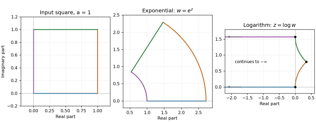
Use the complex logarithm with on the nonzero points of the first-quadrant square. Put . The square bounds give
The two edges meeting at map to the horizontal half-lines and , extending indefinitely to the left. The other edges map to for and for . They meet at .
The angles are preserved at , and . There is finite and nonzero. The origin is a branch point, has no finite logarithmic image, and supplies no fourth finite vertex at which angle preservation could be asserted.
Figure 1.
A square, its exponential annular sector, and its logarithmic image extending to the left
. Details.
Writing gives and . Thus the closed square maps to the annular sector
Its horizontal edges become radial segments and its vertical edges become circular arcs. Each radial tangent is perpendicular to the tangent of its adjoining circle, so the four interior angles remain . Equivalently, the complex derivative is nonzero at every vertex and the map is conformal there.
No region maps onto the entire finite complex plane: is never zero. Its image on is . A fundamental strip such as
maps bijectively onto that punctured plane, because . The half-open strip supplies one representative of each angle; it is not an open domain. An open strip of height omits a ray as well. The missing zero is approached only in the limit .
A conformal map preserves the magnitude and orientation of angles between intersecting smooth curves locally. For a complex holomorphic function, the condition at is : the first-order change rotates and uniformly scales every tangent vector by the same complex factor. This local statement does not require a globally one-to-one map.
Take on the same logarithm branch. At zero, , so the apparent singularity is removable and the closed contour integral is zero. The bank difference is
The circular contributions vanish by the previous estimates with the third power of the logarithm. Consequently
The last integral is , giving
Increasing the logarithm power has converted the desired real integral into a jump across a branch cut, while removing the pole inside the contour.
Use the positive orientation shown in the source: the upper bank runs outwards and the lower bank returns towards one. On those banks the logarithm branch has values and , respectively, with . Their squared difference is . The residue theorem therefore gives
and hence
The large-circle contribution is and the small circle about one contributes , both tending to zero. These estimates justify replacing the closed contour integral by its two cut-bank integrals.
Choose the principal logarithm, so has branch cut . Near zero its Taylor series gives
Thus zero is a simple pole of residue one, and one is a logarithmic branch point. The function is holomorphic on with this branch. Infinity is also a branch point in the extended-plane description; the function's decay there along the cut plane does not make it a single-valued holomorphic function through infinity.
The one-step expected price multiplier under the stated physical probability is . Independence lets the expectation of the product factorize, giving
The same expression follows by summing the four binomial endpoint probabilities times their prices. This is a physical-measure expectation; option replication below uses a separately determined risk-neutral probability.
After three multiplicative steps, upward moves and downward moves give
For , respectively, the prices are . Since the steps are independent, the endpoint probabilities are binomial:
In the displayed ascending-price order they are , , , and . Different paths with the same count of up moves recombine because multiplication by and commutes.
At each time-2 node, replicate one positive put payoff using shares and a current cash deposit . Its two terminal values must satisfy and , with . Thus
For the three nodes the hedge is
At , both child puts expire worthless. At , the child payoffs are and ; at , they are and . Substituting the hedge holdings into both child states verifies those payoffs exactly.
The writer is short the option and therefore holds this positive replicating portfolio to offset the liability. At the lower nodes that means shorting shares and depositing the proceeds together with the option value, rather than buying positive-delta stock. Rebalancing the replicating holdings along the tree is self-financing in the ideal model; the combined short option plus hedge has zero terminal liability in either child state.
At strike , the European put payoff is . In the ascending-price order , its values are
Risk-neutral expectation discounted for three steps gives
The physical probability drops out because the complete two-state tree admits a replicating hedge. The strike is , so the endpoint is out of the money; replacing it by a positive payoff would materially change the price.
Let be the risk-neutral up probability and the one-step risk-free gross return. Discounted asset price must be a martingale, so
The no-arbitrage condition is satisfied, so lies strictly between zero and one. This pricing probability need not equal the actual up frequency .
Financial data show approximate, scale-dependent regularities rather than an exact universal scaling law. Heavy return tails can resemble a power law over an intermediate range, but the fitted exponent, cutoff and range depend on instrument, period and sampling. A straight segment on a log-log plot alone is not enough to establish a power law.
For independent finite-variance increments, variance grows linearly with horizon and typical fluctuations scale as . Central-limit aggregation can make longer-horizon returns more Gaussian even when short-horizon returns are heavy-tailed. Real data can depart from a single self-similar distribution because of volatility clustering, changing regimes, asymmetric responses, intraday seasonality and market microstructure. Apparent different scaling of higher moments may reflect intermittent volatility, but moments estimated from rare tails can also be unstable or may not exist in an idealized model.
Useful tests compare rescaled distributions, structure functions and volatility correlations across several scales, with uncertainty estimates and checks for nonstationarity. Scaling is a valuable approximate modelling guide over a documented range, not proof that one exponent describes every asset and horizon or that historical tail behaviour fixes future extreme losses.

Expand the three increments into their eight monomial products. Exactly one term has every driving-sign index appearing an even number of times: take from , from , and from . Their product is . Every other term leaves an unpaired mean-zero sign. Thus
If the increments were independent, their three zero means would instead give zero. The nonzero third-order moment is therefore a direct demonstration of nonlinear temporal dependence despite vanishing nonzero-lag autocovariances.
Expand into products of the independent mean-zero signs. Each increment is the sum of two monomials, and . At distinct times, no monomial from one increment has exactly the same set of sign indices as a monomial from the other. Every product therefore contains at least one sign to an odd power, whose average is zero. Hence
This argument covers overlapping driver sets at separations one and two, not just the disjoint case at larger separation. At equal times the value is , so the complete autocovariance is . It establishes absence of second-order serial correlation, not independence of returns.
Take the driving signs to be independent across times, with and . Temporal independence of the drivers is an assumption needed in addition to their stated equal one-time probabilities. For ,
As a useful scale check, takes values with probabilities . Its variance is therefore , rather than the unit variance of a single driving sign.

There are unlisted articles, also show them or only show them.