The Harvard spectral classification orders the main stellar classes by decreasing effective temperature: O, B, A, F, G, K, M, from blue to red. Numerical subclasses run approximately from 0, the hotter end of a class, to 9, its cooler end. An A0 star, near 104K, has very strong Balmer series lines; hotter stars ionize much of the hydrogen and cooler stars underpopulate its n=2 level. A G2 star, near 5800K, has weaker Balmer absorption, many neutral and ionized metal lines, prominent Ca II H and K lines and the CH G band. An M5 star, near 3000K, has strong TiO molecular bands, neutral-metal and alkali features, and weak photospheric Balmer absorption.[ref]
Displace a small parcel upward, with negligible heat exchange, rapid pressurebalance, and the same composition as its surroundings. Define the environmental gradient ∇=dlogT/dlogP. An adiabatic ideal gas parcel obeys Pρ−γ=constant and hence T∝P(γ−1)/γ, giving ∇ad=(γ−1)/γ.
The upward displacement has δlogP<0. If ∇<∇ad, the parcel'stemperature changes more negatively than the environment's. At their common pressure it is cooler, denser and driven back down. Therefore the Schwarzschild criterion for stability is
Ionization and dissociation can store compression energy without the full temperature rise of amonatomic gas, lowering the effective adiabatic response in partially ionized outer layers. Radiation pressure tends towards an adiabatic exponent 4/3. These effects, changing composition and degeneracy make the effective exponentposition dependent. The local dynamical exponent is Γ1=(∂logP/∂logρ)s; it equals CP/CV in the simple fixed-composition ideal-gasmodel, but need not do so for an ionizing mixture.
If an envelope has an effective exponent at or below 4/3, its pressure response is soft and sufficiently extensive such regions can promote radial pulsation, envelope instability or mass loss. In the ideal homologous global model, γ=4/3 is marginal and γ<4/3 is unstable to contraction or expansion. A low value confined to a thin outer layer does not by itself prove collapse of the entire star: global stability depends on the pressure-weighted structure. Its location and mass extent matter.
Since U increases with its particle-weighted mean temperature, the equilibrated self-gravitating object has negative heat capacity: adding total energy allows expansion, makes Ω less negative, and reduces U. Conversely, radiating energy permits contraction and raises the internal temperature. This refers to asequence of gravitational equilibria, not to the positive local heat capacity of a parcel at fixed volume.
This is the hydrostatic virial theorem. A nonzero confining pressure retains the right-hand side 4πR3Ps; varying composition, radiation contributions or a spatially varying effective exponent require the integral relation, rather than pulling one γ outside it.
The real carbon cycle has multiple reservoirs and adjustment times, rather than one universally exponential removal process. Air-sea exchange, ocean mixing and carbonatechemistry give a long-lived atmospheric tail; uptake also changes with temperature, circulation and carbon loading. For example, a warming ocean can absorb less additional carbon dioxide, so a fixed b0 omits a potentially positive climate-carbonfeedback. Terrestrial vegetation and soil responses provide further examples. One missing feature is the dependence of carbon uptake on the changing state of the ocean and climate.
The term b1E is the effective atmospheric addition from ongoing emissions. Its coefficient 0.25ppmv/GtC is about half the full-retention estimate 0.47ppmv/GtC, so the model implicitly removes or partitions some emitted carbon promptly. The term −b0(C−C0) represents slower net uptake of the excess by other reservoirs; its relaxation time is b0−1=200years. Both terms have units of ppmv per year.
Thousands of years at constant E0 erase the initial transient, giving
It is the carbon inventory that counts: oxidation adds oxygen to each molecule but does not change the number of carbon-containing molecules. Using 5.15×10¹⁸kg instead changes the estimate by only about one percent. The atmospheric constants are standard Earth estimates, not additional data read from a missing plot.[ref]
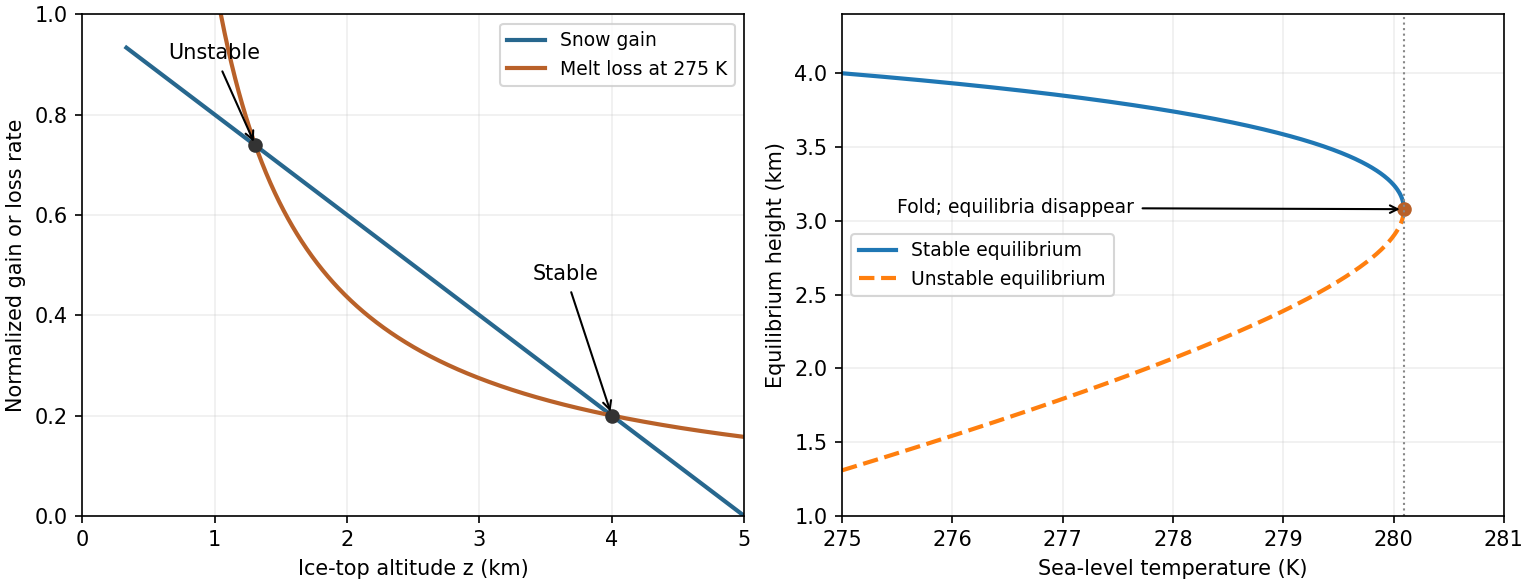
in the normalized rate convention. Using 273K for the Celsius zero instead would give 4.4∘C. The local slope is −0.2+4.43(6)/(22.15)2≃−0.1458km−1<0, as required. Initially z−=1.3083km and zslope≃2.230km, while z+=4km.
As Ts slowly rises, melt loss increases at fixed z, the stable high branch moves downward and the unstable branch upward. They merge at
Beyond the fold the model has no steady coldice cap: its net balance is negative throughout the physical interval and ice shrinks until the assumed law ceases to apply. Quasistatic tracking presumes adjustment is fast compared with the imposed warming, an assumption that deteriorates near the foldas the restoring slope tends to zero. This singular idealized law is not a quantitative real-worldmelting forecast.
The model is singular at z=s/Γ and is not a physical meltinglaw across that boundary. On the relevant interval s/Γ<z<1/β, L decreases hyperbolically and A decreases linearly. Assume a fixed area and positive icedensity, so increasing mass increases z: stability has the same signas F′(z).
This combines a positive allowed interval with a strictly positive discriminant. At the larger root F′<0 and small perturbations restore the ice cap; the smaller root has F′>0 and is unstable. Since
Snow accumulation, melt loss and the ice-cap stability threshold
. The initial curves have an unstable lower intersection and a stable upper intersection. Slow sea-level warming shifts the melt curve until both equilibria meet at afold; all temperatures inside the reciprocal melt law are Celsius. Details.
using cp≃1004Jkg−1K−1. Here temperature in the thermodynamic differential is absolute, g and cp are treated as constant, composition is fixed, and condensation is excluded. Hydrostatic balance alone does not force the atmosphere to be adiabatic; the parcel assumption supplies the extra relation.