
Define the plasma parameter here as the number of electrons in an electron Debye sphere,Some texts instead use neλD3, or its inverse as a coupling parameter. A weakly coupled collective plasma has ND≫1; fluctuations from individual nearby particles are small compared with the collective description.
ND=34πneλD3.
A Coulomb collision means the cumulative deflection or relaxation produced by many small-angle encounters, not necessarily a hard contact between two particles. The Coulomb logarithm lnΛC≃ln(bmax/bmin) summarizes the impact-parameter range, with bmax of order λD. A process is collisionless when its timescale is much shorter than the appropriate collisional relaxation time, or its length scale is much smaller than a corresponding mean free path. It still contains collective interactions.
For fully ionized ions of charge Ze, a thermal electron–ion momentum-relaxation rate has the scalingup to numerical factors depending on the Debye-sphere and collision-time conventions. More explicitly, the Maxwellian rate used below gives νei/ωp≃0.089ZlnΛC/ND, or tcolωp≃11.3ND/(ZlnΛC). Specifying this factor prevents mixing a small coupling parameter with a large Debye-sphere population.[ref]
νei∼ϵ02me1/2(kBT)3/2Znee4lnΛC,tcol∼ZlnΛCωpND,
NRL Plasma Formulary (2019). Fundamental Plasma Parameters and Coulomb Collisions: electron thermal and collision-rate conventions
The electron Debye length is the scale over which a weak electrostatic disturbance is screened. Take the ions as an immobile neutralizing background and the electrons as an isothermal Boltzmann distribution. For a small potential ϕ,Poisson's equation then becomes ∇2ϕ=ϕ/λD2 away from the perturbing source, withA test charge has a screened potential proportional to e−r/λD/r. For fully static screening with mobile ions, inverse squared Debye lengths from all species add; the displayed expression is the electron scale used below.
ne(ϕ)=n0eeϕ/(kBT)≃n0(1+kBTeϕ),ρ≃−kBTn0e2ϕ.
λD=nee2ϵ0kBT.
The electron plasma frequency is the natural collective oscillation frequency when electrons are displaced from a nearly fixed ion background. Displace a uniform electron fluid by ξ along a slab normal. The charge separation produces the restoring electric force −nee2ξ/ϵ0 on an electron. Hence meξ¨=−nee2ξ/ϵ0 andIt sets a response time 1/ωp and the cold unmagnetized electromagnetic cutoff frequency. These collective effects arise from long-range electric fields, even when individual binary collisions are infrequent.
ωp=ϵ0menee2.
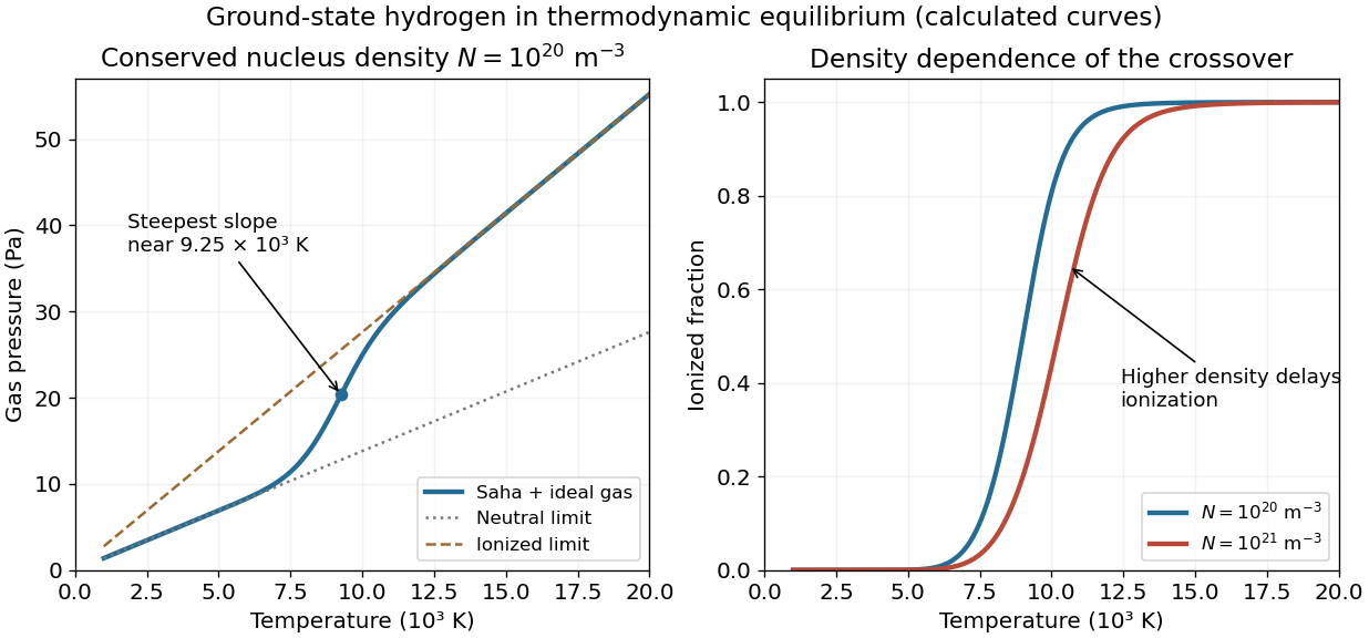
Increasing the conserved nucleus density to 10N multiplies the low-temperature neutral-gas slope and high-temperature ionized-gas slope by ten. However, at a fixed intermediate temperature, x2/(1−x)=S(T)/(10N) is smaller, so a smaller fraction is ionized. The curved transition therefore moves to higher temperature; the new graph is not simply ten times the old graph throughout the crossover.
At a fixed chosen ionization fraction, S(T) must increase tenfold. Locally this requireswhich is of order 103K in this region. Directly evaluating the same Saha equation at 1021m−3 moves the maximum pressure slope from about 9250 to 10560K. The two asymptotic slopes still have ratio two, because each hydrogen nucleus still contributes one particle when neutral and two when fully ionized.
ΔT≃3/(2T)+R/(kBT2)ln10,
Let N=nH+np be the conserved number density of hydrogen nuclei, whether ionized or bound, and x=np/N=ne/N the ionization fraction. The ideal gas pressure counts neutral atoms, free protons and free electrons:At low temperature x≃0 and P≃NkBT. Heating through the ionization region increases the particle count as well as their thermal energy, giving a steeper rise. At high temperature x≃1, so P≃2NkBT and the asymptotic slope is twice the low-temperature slope. There is a smooth ionization crossover, not a pressure discontinuity.
P=NkBT(1+x),1−xx2=NS(T),S(T)=h3(2πmekBT)3/2e−R/(kBT).
The held graph is legible. Representative readings are P(5000K)≃6.8Pa and P(15000K)≃41.4Pa, with readout uncertainties of roughly 0.3–0.5Pa and about 100K. They give N≃P/(kBT) on the neutral branch and N≃P/(2kBT) on the ionized branch, respectively. Both are consistent withThe error is a conservative graph-reading estimate, not a fitted experimental confidence interval.
N≃(1.0±0.05)×1020m−3.
For that density, the Saha equation gives x≃0.50 at 9000K, x≃0.81 at 10000K, and x≃0.9992 at 15000K. Differentiating the ionization relation givesThe calculated maximum slope occurs near 9.25×10³K, consistent with the source's visibly steepest region at roughly (9.3±0.4)×103K. This checks the actual slope rather than identifying it without justification with exactly half ionization.
x′=2−xx(1−x)(2T3+kBT2R),P′=NkB(1+x+Tx′).
Taking the neutral ground-state gas as the zero of internal binding energy, the matter energy density is translational kinetic energy plus ionization energy:At 15000K, with R=13.6eV, these terms are about 62 and 218Jm−3, givingRest energies are excluded. A separate equilibrium radiation field, if the gas were in a blackbody cavity, would add its own radiation energy density; it is not part of this gas-only estimate.
u=23NkBT(1+x)+NxR.
u≃2.8×10²Jm−3.
Assume ideal, nondegenerate particles in local thermodynamic equilibrium, ground-state atomic hydrogen, no molecules, and a common temperature. Let λj=h/2πmjkBT be the thermal de Broglie wavelength. Choose zero energy for a separated stationary proton and electron, so a neutral atom has ground-state energy −R. The classical chemical potentials areChemical equilibrium for H⇌p+e requires μH=μp+μe. Rearranging givesIncluding electron and proton spin degeneracy, ge=2, gp=2 and gH=4 when hyperfine splittings are neglected. Hence the statistical factor is one. Also mH≃mp, so λH3/λp3≃1. Charge neutrality gives np=ne, and thereforeThis is the specified ground-state Saha equation. Keeping excited atomic partition functions or a different spin-counting convention can change a prefactor, so its convention must be stated rather than silently adding a factor of two. The left side has dimensions of a number density, not a dimensionless electron-to-neutral ratio.
μe=kBTlngeneλe3,μp=kBTlngpnpλp3,μH=−R+kBTlngHnHλH3.
nHnenp=gHgegpλe3λp3λH3e−R/(kBT).
nHne2=h3(2πmekBT)3/2exp(−kBTR).
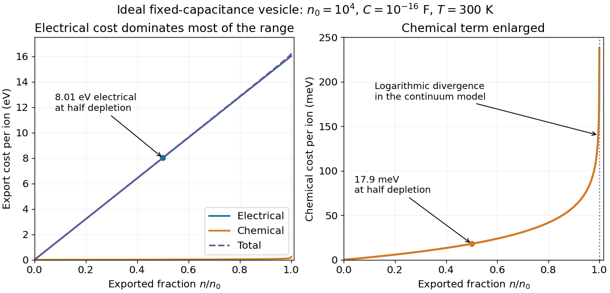
Use the initial equal-concentration, zero-potential reference, or equivalently quote component changes relative to the initial electrochemical equilibrium. At n=n0/2=5000, with C=10−16F,At room temperature T=300K, the chemical component isThe electrical cost dominates by about 447. The associated change in membrane potential is −ne/C=−8.01V. Such a large voltage is a consequence of the ideal fixed-capacitance, perfectly impermeable model; an actual lipid membrane would not generally remain intact and nonconducting over this entire extrapolation.
ΔGelec=C5000e2=1.28×10⁻¹⁸J=8.01eV.
ΔGchem=kBTln2=2.87×10⁻²¹J=0.0179eV.
The electrical component is a straight line through zero, ne2/C. The chemical component, kBTln[n0/(n0−n)], starts at zero, increases convexly, and diverges as n→n0− because the remaining internal concentration vanishes. Their sum lies above both: nearly electrical over most of the stated range, but eventually diverging with the chemical term. For a nonzero initial equilibrium potential, the separate absolute electrical and chemical components have opposite constant offsets; the total curve and the quoted changes remain the same. The final few ions require a discrete-particle treatment rather than a literal continuum divergence.
Use number concentrations and write the electrochemical potential of a sodium ion as μ=μ∘+kBTlnc+eψ. Define the inward sodium-motive force as available work per positive charge for transport from outside to inside. With Vm=ψi−ψo,Its negative is the signed inward free-energy cost per charge; stating this direction removes a common sign ambiguity.
ENa=eμo−μi=ekBTlncico−Vm.
Long-open sodium channels establish electrochemical equilibrium, kBTln(ci0/co)+eVm0=0. This does not generally require equal concentrations: impermeant counterions can support a nonzero equilibrium membrane potential. Let n0=ci0V. For a large fixed-concentration external reservoir, after pumping n ions out, ci(n)=(n0−n)/V and Vm(n)=Vm0−ne/C. The sodium export cost from a capacitive vesicle for exporting another ion isThe initial-equilibrium relation was used in the last step. The first term is the incremental electrical cost and the second is the change in chemical cost from their initial balanced values.
ΔGNa(n)=kBTlnn0−ncoV−eVm0+Cne2=Cne2+kBTlnn0−nn0.
If the intended initial reference is uncharged with Vm0=0 and ci0=co, then n0=coV and the requested form in the listed variables isThat equal-concentration reference is an additional assumption. For example, ci0=2co and Vm0=−(kBT/e)ln2 also give zero initial sodium flux, but a different ion inventory. Thus the open-channel condition alone cannot determine n0 from coV. If concentrations are molar rather than number densities, use the corresponding Avogadro constant conversion and RT for molar free energies. Treating the capacitor charge discretely gives a charging-energy increment (n+1/2)e2/C rather than the differential ne2/C; the distinction is negligible for the thousands of ions used next.
ΔGNa(n)=Cne2+kBTlnco−n/Vco,0<n<coV.
Cells interconvert several forms of free energy. Chemical concentration differences and the chemical potentials of metabolites can drive reactions, including ATP hydrolysis. The usable free-energy difference is that between reactants and products under the actual cellular conditions; breaking a chemical bond alone does not release energy without the rest of the reaction. Oxidation-reduction reactions transfer electrons down an electrochemical potential difference and can drive ion pumping in an electron transport chain. Light absorption can create excited states and charge separation in photosynthesis, eventually supporting chemical synthesis.
An electrochemical gradient stores free energy in both an ion concentration difference and a membrane potential. Chemiosmosis couples downhill ion flow to ATP synthesis by chemiosmosis; ATP-powered pumps can run the conversion the other way. Molecular motors and other mechanochemical enzymes convert chemical free energy into mechanical work or elastic strain, while ion gradients can also power transport and rotary motion. These couplings conserve total energy but dissipate some free energy as heat. Equilibrium thermal fluctuations alone cannot sustain directional work without a maintained nonequilibrium resource.
Under the simplest interpretation, each spot contains two equally bright, independently bleaching green fluorescent protein emitters. Losing one halves the fluorescence and losing the other removes it. A stable protein dimer carrying one active label per subunit is consistent with this result. The conclusion is two active emitters in the observed spot; it does not by itself rule out unresolved coincident proteins, incomplete fluorescent maturation or blinking. Permanent membrane binding makes loss by dissociation less plausible, but lateral motion out of the observation region would still need experimental control.[ref]
Membrane-protein photobleaching counting study (2007). stepwise photobleaching as a subunit-counting measurement and its labeling assumptions
Let their independent photobleaching times be TA,TB∼Exp(kb). Then t1=min(TA,TB) has rate 2kb, while the memoryless remaining lifetime t2−t1 has rate kb and mean 1/kb, matching the stated single-emitter calibration. The two-emitter photobleaching completion time is the maximum, not one single exponential and not a sum of two equal-rate exponential variables. Its cumulative distribution function isDifferentiating gives its probability density function:with zero density for t<0. It integrates to one, and its mean is 1/(2kb)+1/kb=3/(2kb). This uses two active fluorophores at the start of observation, constant illumination and independent irreversible bleaching with the calibrated rate.
P(t2≤t)=P(TA≤t,TB≤t)=(1−e−kbt)2(t≥0).
ft2(t)=2kbe−kbt(1−e−kbt)=2kb(e−kbt−e−2kbt),t≥0,
The excitation rate in the weak, unsaturated fluorescence regime is proportional to the time-averaged squared electric field amplitude. Thus the illumination profile relevant to excitation isThe amplitude decay length 1/κ is twice the intensity decay length. This profile is often called the evanescent excitation intensity; it does not imply a propagating normal energy flux through an ideal lossless totally reflecting interface.
I(y)=I(0)e−2κy=I(0)e−y/dI,dI=2κ1=4πng2sin2θ−nw2λ0.
Total internal reflection fluorescence microscopy restricts excitation to a shallow layer adjacent to the glass, typically on the scale of hundreds of nanometres for visible wavelengths and suitable angles. Fluorophores near the basal cell membrane are excited while much of the cytoplasm and bulk solution remain dark. The resulting reduction in out-of-focus fluorescence and autofluorescence improves the signal-to-background ratio for individual molecules, allows camera-based parallel observation, and reduces unnecessary excitation of deeper regions. Its limitation is the same selectivity: it does not image arbitrary molecules deep inside a cell. This near-interface selectivity was directly demonstrated in cell–substrate contact imaging.[ref]
Cell-substrate TIRF demonstration (1981). evanescent excitation and reduction of fluorescence background at cell–substrate contacts
Let the interface be y=0, with glass at y<0 and water at y>0, and choose x parallel to the incident beam's tangential component. Define k=ω/c as the vacuum wavenumber, with glass and water refractive indices ng and nw. Continuity of phase along the interface fixes kx=kngsinθ. In water, the dispersion relation is kx2+ky2=k2nw2, so above the critical angle,Choose the positive imaginary part because a field growing exponentially into the water would be unphysical. The evanescent field in total internal reflection is thereforeIt propagates in phase parallel to the interface but decays normally. Here E0 is the transmitted field amplitude at the interface; relating it to the incident amplitude requires the appropriate polarization-dependent Fresnel equations. If the symbol k instead denotes the incident glass wavenumber, replace every vacuum k in the formula by k/ng; equivalently kx=ksinθ and κ=ksin2θ−(nw/ng)2. This states the wavenumber convention left implicit in the source.
ky2=−k2(ng2sin2θ−nw2),ky=iκ,κ=kng2sin2θ−nw2>0.
E(x,y,t)=E0exp[i(kngsinθx−ωt)]exp[−kng2sin2θ−nw2y].
The protein primary structure is the ordered protein sequence along a polypeptide, from its N-terminus to its C-terminus. In cells, information in a DNA coding sequence is copied into messenger RNA by transcription. During translation, the ribosome reads successive three-base codons; transfer RNA molecules match these by their anticodons and supply the corresponding amino acids. The genetic code is degenerate: different codons can encode the same amino acid. A start establishes the reading frame and a stop terminates translation. Peptide bonds link the amino acids into the backbone, leaving chemically different side chains. Thus the sequence specifies the order of side-chain interactions, rather than a literal coordinate list for the folded molecule.
Protein secondary structure describes local backbone arrangements. An alpha helix is stabilized by a regular pattern of backbone hydrogen bonds, typically between the carbonyl of residue i and the amide of residue i+4. Beta sheets assemble extended strands through inter-strand hydrogen bonding, with parallel or antiparallel strand orientations. Turns and loops connect these elements; not every region belongs to a helix or sheet. The peptide bond is approximately planar, while backbone torsion angles provide conformational freedom subject to steric restrictions.
Protein tertiary structure is the complete three-dimensional organization of one chain, often arranged into protein domains. Protein quaternary structure describes the organization of multiple chains in an assembly. Soluble globular proteins often bury nonpolar side chains and expose polar ones; membrane proteins can instead expose hydrophobic surfaces to the surrounding lipid. Other stabilizing interactions include hydrogen bonds, electrostatic interactions, Van der Waals forces and sometimes covalent disulfide bonds. These competing contributions define active sites, binding pockets and mechanically useful structures; folded proteins are dynamic ensembles, not perfectly rigid objects.
The connection from sequence to structure is thermodynamic and kinetic. Folding usually decreases the chain's conformational entropy, but favorable interactions and changes in solvent entropy, including the hydrophobic effect, can lower the total Gibbs free energy. Under suitable conditions the native ensemble is favored over unfolded alternatives. A change in sequence can therefore change the balance of accessible conformations and alter folding or function. Reversible refolding of a denatured protein in an appropriate environment demonstrates that the sequence can contain the information needed for its native structure.[ref]
Protein-chain folding principles (1973). thermodynamic hypothesis and refolding experiments, pp. 223–225
The environment is part of the specification: temperature, pH, ionic conditions, ligands and post-translational modifications matter. Molecular chaperones can prevent aggregation and help chains escape kinetic traps without providing a residue-by-residue structural template. Some sequences are intrinsically disordered proteins or disordered regions, and some require partners for a stable fold. Thus primary structure strongly constrains structure, but does not guarantee one unique rigid shape independent of conditions.
There are three physical controls: alter the energy splitting, alter the temperature, or drive the spin populations away from thermal equilibrium.
Increasing the static magnetic flux density increases ΔE=ℏγB, and hence the equilibrium nuclear spin polarization approximately in proportion to B/T. High-field magnetic resonance imaging exploits this for greater available magnetization and potentially finer spatial or temporal resolution. The disadvantages include more demanding magnets, stronger susceptibility-related distortions, and harder radio frequency field uniformity and power management. A direct experimental comparison of head imaging at 7 T and 4 T measured both the signal gain and the RF penalties.[ref]
High-field MRI comparison (2001). head-imaging measurements of signal-to-noise, RF power and field homogeneity
Lowering the spin sample's temperature increases its equilibrium polarization at fixed B. Cryogenic preparation of an imaging agent can exploit this, often assisted by dynamic nuclear polarization, followed by rapid dissolution and transfer for hyperpolarized magnetic resonance imaging. This offers a much larger signal from dilute nuclei than room-temperature equilibrium, but requires preparation hardware, rapid transfer and acquisition before spin-lattice relaxation erases the polarization. Cooling an RF receiver reduces electronic noise, but does not itself change the nuclei's population ratio; nor does this argument propose cooling living tissue to cryogenic temperatures. The demonstrated dissolution method combines low temperature, magnetic field and microwave-assisted polarization transfer, so its gain must not be attributed to cooling alone.[ref]
Dissolution dynamic nuclear polarization demonstration (2003). solid-state polarization and rapid dissolution preserving enhanced nuclear polarization
Driving transitions with a resonant radio frequency field changes the longitudinal populations without changing B or the bath temperature. A π pulse interchanges the populations; saturation equalizes them. Inversion recovery then measures or exploits their return toward equilibrium, Mz(t)=M0(1−2e−t/T1) after an ideal inversion, providing tissue contrast and signal nulling. Advantages are selective contrast and control within an ordinary scanner; costs include reduced signal, extra acquisition time, RF energy deposition and sensitivity to pulse errors. Such RF pulses alone cannot create a polarization magnitude greater than the available equilibrium value. Genuine nonthermal enhancement instead transfers polarization from another spin reservoir, for example electron spins in dynamic nuclear polarization or optically polarized noble gases in lung imaging; its transient and preparation constraints differ from ordinary RF inversion.[ref]
Dissolution dynamic nuclear polarization demonstration (2003). introductory account distinguishing optical pumping, spin-order transfer and DNP from thermal polarization
Write x=ΔE/(kBT) and r=N↑/N↓=e−x. Since N=N↑+N↓, eliminate the individual populations:The Taylor expansion e−x=1−x+O(x2) gives the same result, and the odd expansion of the hyperbolic tangent yieldsEquivalently, N↑≃(N/2)(1−x/2) and N↓≃(N/2)(1+x/2). Their sum is still N. The negative sign follows directly from the stated higher-energy up-state population, and does not mean a negative magnitude of the equilibrium magnetization.
NN↑−N↓=r+1r−1=e−x+1e−x−1=−tanh2x.
NN↑−N↓=−2x+O(x3)≃−2kBTℏγB.
Take room temperature as T=300K. With the supplied gyromagnetic ratio, reduced Planck constant and Boltzmann constant,soAt 293K the ratio is 1.05×10⁻⁵; the room-temperature convention makes only a small difference. The corresponding fractional nuclear spin polarization has magnitude about five parts per million. The source's negative sign convention assigns the label up to the higher-energy state; it should not be confused with the lower-energy magnetic moment aligned with a positive proton magnetic field.
ΔE=(1.054×10⁻³⁴)(2.675×10⁸)(1.5)=4.23×10⁻²⁶J,
kBTΔE=(1.380×10⁻²³)(300)4.23×10−26=1.02×10⁻⁵.
Use the linear-quadratic radiobiology model, independent fractions with complete inter-fraction repair, and no tumour repopulation. For N fractions of dose d, the logarithmic cell kill is N(αd+βd2). Dividing by α defines the biologically effective dose,For the tumour, the original schedule gives 26(2)(1+2/10)=62.4Gy10. A 3Gy fraction contributes 3(1+3/10)=3.9Gy10, so precisely 62.4/3.9=16 such fractions give the same tumour biologically effective dose. The physical total dose changes from 52 to 48Gy.
BED=Nd(1+α/βd).
For the specified normal-tissue α/β=3Gy, the original and altered schedules giveThus the normal-tissue model predicts an increase of 9.33Gy3, or about 10.8%, despite the smaller total physical dose. The smaller normal-tissue α/β makes increasing fraction size relatively more costly. These are comparisons within the source's hypothetical radiobiological model and equal-dose geometry, not individualized treatment prescriptions.[ref]
BEDold=52(1+32)=86.7Gy3,BEDnew=48(1+33)=96.0Gy3.
Linear-quadratic fractionation study (1989). BED formulation and dependence on fraction size and alpha/beta
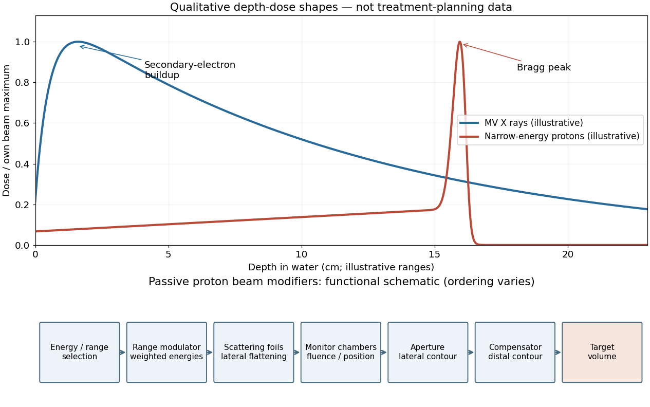
A passively scattered proton therapy beam uses distinct devices to control lateral spread, range and distal shape. The lower panel of the figure gives a functional schematic; the exact ordering varies among beamlines. An energy selector or range shifter sets the maximum range. A stepped range-modulation wheel or ridge filter gives a weighted collection of proton energies, forming the spread-out Bragg peak. One or more scattering foils broaden the narrow beam; a double-scattering system can improve lateral uniformity. Ionization chambers monitor delivered fluence and position. A patient-specific aperture or collimator blocks unwanted lateral regions. A shaped range compensator makes the remaining range vary across the field, matching the distal target boundary. Their effects must be combined: lateral collimation alone cannot flatten the depth distribution, and an energy modulator alone cannot set the lateral contour.[ref]
Passive proton double-scattering study (1977). original experiments and design: blocking the central peak followed by rescattering to flatten a large field
For a megavoltage X-ray beam, the surface absorbed dose is below the subsurface maximum. Photons generate energetic secondary electrons, mainly through Compton scattering; the downstream electron fluence initially builds up until approximate charged-particle equilibrium is established. Beyond this buildup region, decreasing primary photon fluence, scattering and geometric spreading make the depth-dose curve fall gradually. A penetrating photon beam has a substantial exit dose.
A nearly monoenergetic proton beam deposits a moderate entrance dose, then a sharp Bragg peak near the end of its range. As nonrelativistic protons slow, their electronic stopping power rises approximately as 1/v2 over the relevant part of the track. Once the protons stop, the dose falls steeply. Range straggling and energy spread broaden the peak; nuclear interactions add a smaller nonideal tail, so an exact hard cutoff is an idealization. Superposing appropriate incident energies produces a spread-out Bragg peak covering an extended target.[ref]
Proton depth-dose proposal (1946). pp. 487–489, increasing specific ionization near the end of range
The label MV for an X-ray treatment beam specifies the nominal accelerating potential of the electron accelerator. Its bremsstrahlung beam is a broad photon energy spectrum with an endpoint of order eV, not a monoenergetic beam whose individual photons all carry the quoted numerical energy. Proton therapy beam energies can instead be specified directly in MeV per incident proton.


In the ideal unscattered coincidence model, let a positron annihilation occur at position s on a coincidence line of response connecting detectors A and B. Its two oppositely directed photons must both survive. Their independent attenuation factors multiply:The source position cancels because the complementary path integrals span the whole chord. In a uniform slab of chord length L, the same argument is e−μse−μ(L−s)=e−μL. Therefore attenuation correction requires the full linear attenuation coefficient map along the chord, but not the depth of the particular annihilation along that chord. This argument addresses attenuation of true PET coincidences; scatter, random coincidences and detector efficiency need their own corrections.
Pcoinc(s)=exp[−∫Asμ(ℓ)dℓ]exp[−∫sBμ(ℓ)dℓ]=exp[−∫ABμ(ℓ)dℓ].
A CT number is a dimensionless relative attenuation measure, conventionally H=1000(μCT−μwater,CT)/μwater,CT. The X-ray spectrum used in computed tomography has an effective energy far below 511keV and is polychromatic. Its photoelectric absorption contribution depends strongly on composition, whereas water and soft-tissue attenuation at the positron emission tomography energy is mainly Compton scattering. Thus a CT number is neither a 511keV linear attenuation coefficient nor an energy-independent mass attenuation coefficient.
The usual conversion calibrates a piecewise linear or bilinear relation between CT numbers and μ(511keV). The air–water branch models predominantly density differences in lung and soft tissue; a separate water–bone branch accounts for the different energy dependence of mineralized tissue. The calibration depends on the computed tomography spectrum. After geometric registration, the resulting linear attenuation coefficient map is forward projected along each coincidence line of response to obtain exp(∫μ511ds). If a mass coefficient is stored, its conversion to a linear coefficient must also include mass density. Unusual high-atomic-number materials can violate the simple tissue calibration, so the conversion is a physical material model, not a universal arithmetic rescaling.[ref]
CT-based PET attenuation correction study (1998). original study: segmentation, scaling and hybrid conversion from CT energies to 511 keV
[ref] There are unlisted articles, also show them or only show them.