Define fractional ionization as and use electrical neutrality. For and , . Thus the density form of the Saha equation requires
Solving this monotone equation, conveniently after taking its logarithm, gives
The thermal energy is only about of the eV ionization energy. Ionization is not decided by setting : the high-energy tail and the large translational state-count factor in chemical equilibrium allow a residual ionized fraction at a much lower temperature. This is the equilibrium estimate for the stipulated density and fraction, without inferring an expansion age from it.
Assume a dilute nondegenerate ideal mixture in thermal and chemical equilibrium, electrical neutrality , and ground-state hydrogen only. Choose the zero of internal energy as a separated proton and electron, so the atom has energy . Its single-particle partition function contains :
Their ratio has one remaining power of . Neglecting binding mass in makes the translational mass factor . For unresolved ground-state spin states, : including proton spin gives , or omitting it consistently gives . The given law of mass action therefore yields
This is the Saha equation with the degeneracy convention used by the source. Equivalently .
Using the replacement prescribed in the question, , gives
The number of electrons in a Debye sphere is consequently
A useful check eliminates : with and , and .
Having substantially fewer than one electron in this sphere shows that the classical many-particle Debye-screening picture is not applicable. It does not exclude collective plasmons in a degenerate electron gas. A proper zero-temperature Thomas-Fermi screening calculation uses and gives , rather than literally replacing by . The boxed count follows the source's stated prescription and exposes its physical limitation.
For a nonrelativistic, three-dimensional ideal electron gas with spin degeneracy two,
Dividing gives
Write the density-independent coefficient as . From , . In this free-electron model,
The result uses the stipulated energy ratio, rather than substituting a separately tabulated aluminium density or plasmon energy.
The Debye length is the distance over which a small, slowly varying electrostatic potential is screened by mobile thermal charges. For classical electrons in a weak potential , their Boltzmann distribution gives
Take fixed singly charged ions of density . Then , and Poisson's equation outside a test charge becomes , with
The screened point-charge potential is proportional to . The derivation assumes nondegenerate statistics and . Mobile ions would add their own contribution to ; the expression here is the electron screening length.
Treat the ions as a stationary neutralizing background and displace the cold electrons by a small longitudinal distance . Their electric polarization is , so the restoring electric field is . The electron equation of motion is
For , the oscillatory velocity is . Hence
The longitudinal mode exchanges electron kinetic energy and electrostatic field energy like a harmonic oscillator, whose mean kinetic and potential energies are equal over a cycle. This is a time-average statement for the coherent oscillation, not thermal equipartition with .
Use eV and eV. The nonrelativistic beam speed and cross-sectional area are
Here , , and the exponential in the requested threshold is . With ,
Converting beam density to the magnitude of its electric current gives
This is an order-of-magnitude estimate from the source's asymptotic formula. The numerical hierarchy is only moderate: . Retaining the background slope at instead gives about A as a sufficient positive-slope current at that chosen velocity. The difference quantifies the sensitivity of the exponential-tail approximation; an exact kinetic instability threshold requires the dispersion relation. The requested estimate is therefore on the scale of tens of kiloamperes, rather than a precisely determined current.
At , the beam's positive slope is , while the background slope has magnitude . Thus a nonnegative total slope at this velocity requires
Approximating the background slope by its value at yields
Equality is the local marginal-slope condition; strict inequality gives positive resonant drive in this approximation. The numerical is of order unity and can change when the resonant velocity is optimized or the full wave dispersion is retained.
Replacing by in the exponential is controlled only if , in addition to . The two width inequalities alone do not guarantee that extra condition far out on a Maxwellian tail. The preceding unapproximated slope inequality remains available when it is not satisfied.
For the shifted beam Maxwell-Boltzmann distribution,
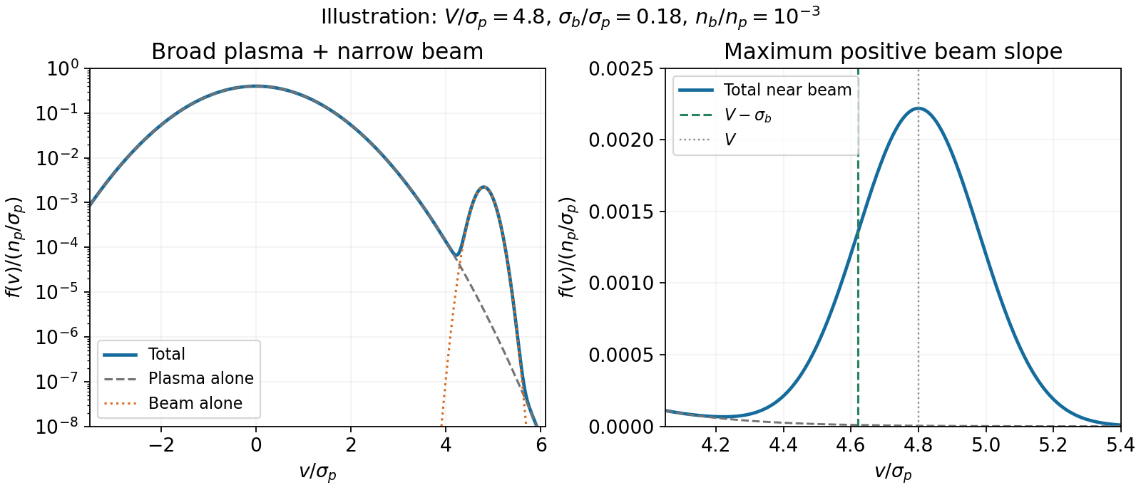
On the rising flank put . The positive slope is proportional to , whose derivative is . Its unique positive maximum is at , giving
This is the region where beam drive can most readily overcome the negative plasma slope when that background changes little over the narrow beam width. It is an estimate for the first resonant unstable wave, not a proof that every beam-plasma dispersion relation has its exact marginal phase velocity at this value. Both the total slope and the real dispersion relation determine the exact marginal mode.
Define the one-dimensional thermal widths and . Normalize each velocity distribution to its electron number density:
The total is . It consists of a broad peak centred at zero and a much narrower displaced beam near , with . Their areas, rather than their peak heights, are and . A weak narrow beam can make a positive-slope region on its low-velocity side even while contributing little to the total density.
Figure 1.
Broad plasma Maxwellian and a narrow displaced electron beam
. Illustrative normalized widths and density ratio are used to display the beam on the background tail. The marked V−sigma_b is the point of maximum positive beam slope, not a universal exact marginal-mode velocity. Details.
Landau damping is the collisionless decay of a plasma wave through resonant energy exchange with particles whose velocity is close to the wave's phase velocity . Particles slightly slower than the wave tend to gain energy from it; particles slightly faster can give energy to it. For the decreasing resonant part of a Maxwell-Boltzmann distribution, the net transfer is from the wave to the electrons, so the wave amplitude decays.
In the linear Vlasov equation description this is collisionless phase mixing, not a requirement for frequent particle collisions. Fine-scale structure develops in the velocity dependence of the perturbation even while the macroscopic electric field decreases. The resonant contribution to the growth rate has the sign of at a positive wave phase velocity: a negative slope produces damping, whereas a sufficiently positive slope can drive an instability. A population comparison must be local to the resonance; merely counting all particles faster and slower than the wave is not the criterion.
For constant and no drift, particle conservation and Fick's first law give the one-dimensional diffusion equation . For ,
so direct substitution verifies the equation for . The Gaussian integral fixes the normalization:
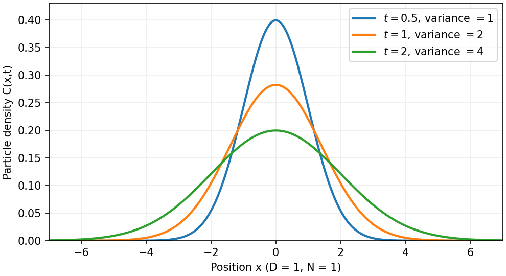
This is the heat kernel for a point release, with in the distributional limit. It remains centered at zero while its width grows as and its peak falls as . To compute the second moment, set :
using over the whole real line, obtained by integration by parts.
If the mean number of independent unbiased jumps in time is , conditioning on gives . Matching it to the continuum diffusion result yields
For fixed-magnitude steps , . The equality of second moments also holds for Poisson jump times independent of the increments; a Gaussian continuum approximation additionally requires many steps and finite step variance.
Figure 1.
Spreading of a normalized one-dimensional diffusion packet
. Analytic Gaussian profiles with N=1 and D=1 at three illustrative times have fixed unit area, peak proportional to inverse square root of time, and variance 2Dt. Details.
Let be the particle number density, the conservative potential energy and the applied force. In the overdamped regime a viscous drag coefficient gives drift velocity . Combining this drift with Fick's first law gives the number flux
At thermal equilibrium, the Boltzmann distribution is , so . Setting its net flux to zero yields
This is the Einstein diffusion relation. The derivation assumes a dilute equilibrium suspension, uniform temperature, linear drift response and a well-defined long-time diffusion coefficient. With a nonzero conservative force, the full transport equation includes drift; the force-free equation in the next section describes spreading without that drift.
Write the one-dimensional random walk endpoint as , starting at the origin. Assume unbiased, independent increments, each with and . Expanding the square gives
Independence makes each cross expectation . Consequently
Uncorrelated increments with the same second moments would suffice. Unbiasedness alone does not remove correlations: persistent or anticorrelated steps need not satisfy this result. The symbol is already the mean-square step size, with units of length squared.
Let be the probability that an ATP-waiting state has not yet bound a substrate molecule. A constant bimolecular binding coefficient at fixed ATP concentration gives a pseudo-first-order hazard . Thus , , and the waiting-time distribution is
The probability density function starts at and decreases exponentially. Increasing shortens the waiting time in inverse proportion. This supports one rate-limiting ATP-binding event before the associated motion, rather than a concentration-independent chemical delay.
For the second delay, consider sequential independent first-order transitions . Their dwell times have exponential distributions. The total waiting time is their sum, so convolution gives
It is normalized, symmetric under exchange of , and has
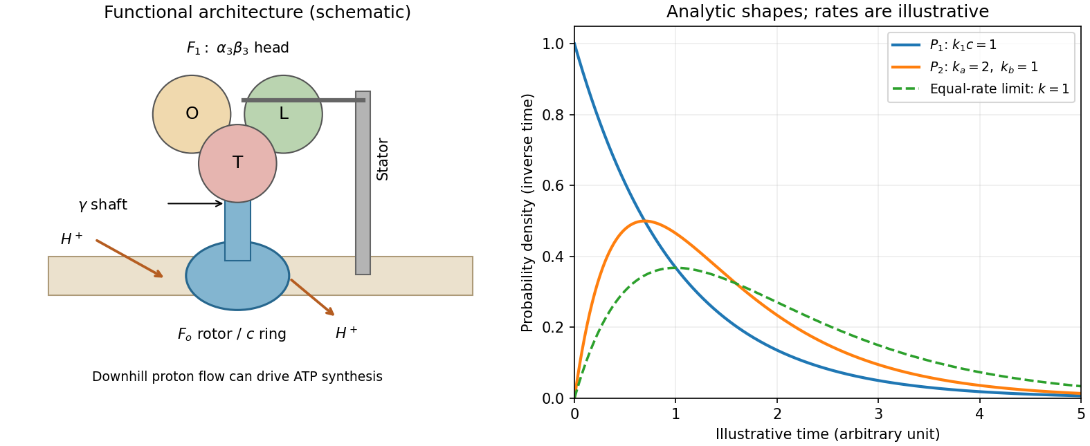
Unlike one exponential delay, it vanishes at , rises initially as , reaches a maximum at and eventually decays at the slower rate. For equal rates the continuous limit is , an Erlang distribution with mode . If one rate is much faster than the other, the observed long-time behavior approaches one exponential. The sketch in the preceding section displays these shapes using arbitrary specified rates.
The simplest catalytic cycle compatible with the fits therefore contains an ATP-dependent binding delay and at least two resolvable ATP-concentration-independent kinetic events. Hydrolysis, product release and conformational changes are possible microscopic assignments, but the two-rate fit alone does not uniquely identify them or the order of and . If each complete cycle contains these three waits and step durations are negligible, its mean duration is and the mean revolution rate is the inverse of three times this duration. Multiple catalytic sites can cooperate during that cycle.
TODO: the source PDF's stepping plot is absent. Its individual substep angles, numerical timings and the mapping of plotted dwell labels onto the larger or smaller angular movement cannot be read. The surviving text establishes only the total step and the existence of a larger and a smaller substep. No numerical rate, missing angle or plotted label is inferred from a different experiment. The distribution derivations and the concentration-dependence inference above are independent of that illustration.

ATP synthase couples downhill proton motion across a cell membrane to synthesis of ATP from ADP and inorganic phosphate. Its membrane-embedded sector contains an subunit with offset proton-access half-channels and a rotating -subunit ring. Reversible protonation of sites on the ring permits rotation relative to the stationary subunit. The central rotor transmits this motion through the shaft to the soluble head. A peripheral stator holds the head relative to the membrane sector. The common bacterial schematic has an head, catalytic sites mainly on the three subunits, and a central rotor; accessory stator components depend on the organism.
The binding-change mechanism cycles the catalytic sites between open, loose-binding and tight-binding conformations. Rotor orientation changes their affinities for ADP, phosphate and ATP; the sites operate out of phase. Tight binding favors formation of bound ATP, and mechanical rotation changes the conformation to permit product release. In the ideal tightly coupled cycle, one revolution gives three catalytic turnovers:
The proton count is not universally fixed: an ideal ring with proton-carrying subunits gives protons per revolution and protons per synthesized ATP, before additional transport costs.
For a proton moving from side 1 to side 2, its molar electrochemical potential change is
The chemical gradient and membrane electric potential difference together supply the proton-motive force. Synthesis requires the proton free-energy release to meet the positive Gibbs free energy of ATP synthesis. The coupling is reversible: isolated supplied with ATP can hydrolyse it and rotate its shaft, while the intact enzyme can use hydrolysis-driven rotation to pump protons against their gradient. The sketch is structural and schematic; it does not reconstruct the absent stepping trace.
Figure 1.
ATP synthase architecture and the two derived dwell-time distributions
. The structural panel shows a membrane rotor, shaft, stator and three catalytic sites. The distribution panel uses explicitly illustrative dimensionless rates, not values read from the absent source stepping plot. Details.
Protein primary structure is the ordered amino acid sequence of a polypeptide, linked by covalent peptide bonds. The approximately planar peptide bond restricts local geometry, while backbone torsion angles give conformational freedom subject to steric exclusion. Protein secondary structure comprises local backbone arrangements, especially the alpha helix, with backbone hydrogen bonds between residues and , and the beta sheet, whose strands are joined by backbone hydrogen bonds. Turns and loops connect these elements. Protein tertiary structure is the full three-dimensional organization of a single chain, often including several protein domains. Protein quaternary structure is the arrangement of multiple chains in a protein complex.
Protein folding is governed by the Gibbs free energy of the chain together with its solvent, not by the chain's energy alone. Folding reduces the chain's conformational entropy, but can gain solvent entropy through the hydrophobic effect, burying nonpolar side chains away from water. Favorable hydrogen bonds, Van der Waals forces, electrostatic interactions and sometimes covalent disulfide bonds stabilize particular structures. Steric repulsion prevents atomic overlap. At fixed temperature and pressure, the native ensemble is favored when its total is lower than competing ensembles. The balance depends on the solvent, pH, salt and ligands. Molecular chaperones help avoid aggregation or kinetic traps; a stable fold is not a perfectly rigid conformation, and some proteins have disordered regions.
For a soluble globular protein, a typical pattern is a nonpolar core and a polar, hydrated surface. A transmembrane protein instead presents nonpolar side chains to the hydrocarbon interior of the lipid bilayer. Membrane-spanning alpha helices satisfy their polar backbone groups through internal hydrogen bonds; a roughly membrane-thickness helix commonly contains about twenty residues, depending on tilt and bilayer thickness. Multiple helices can enclose polar channels or binding sites. Membrane-spanning beta barrels likewise expose mainly nonpolar groups outward towards lipid while arranging backbone hydrogen bonds between strands and often lining an aqueous pore with polar groups. Exposed loops and domains contacting water can resemble soluble proteins. Not every membrane-associated protein spans the membrane: peripheral attachment and lipid anchoring are distinct possibilities.
The organizing distinction is the environment of each surface: water favors accessible polar groups, while the membrane core favors outward-facing nonpolar groups. Buried polar groups can still be essential to a transport pathway or catalytic site.
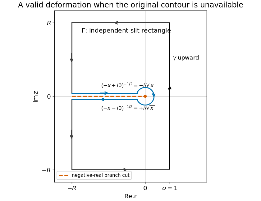
TODO: the original closed-contour drawing is absent from the source. The following independent Bromwich contour deformation establishes the required discontinuity relation without asserting the missing drawing's exact geometry. Orient the vertical line upward, as required by the positive imaginary answer in the next part, and use the principal square root, .
Close a truncated vertical line to the left with a rectangle, slit it along the negative real axis, and exclude a small circle about zero. The integrand is holomorphic inside that slit domain, so the boundary contour integral is zero. Horizontal boundary integrals are : integrating along gives a bounded factor while . The left boundary contributes , and the small circle contributes . All vanish in the indicated limits.
At with , the upper and lower bank values are respectively and . The boundary follows the upper bank toward zero and the lower bank away from zero. Their combined contribution is . Hence
The vertically improper integral converges conditionally; these estimates also justify the contour limit. Reversing the vertical orientation reverses its sign.
Figure 1.
An independently chosen slit-rectangle contour relates the upward Bromwich integral to the square-root branch jump
. Details.
The square-root branch points are zero and infinity. At zero the local behavior is ; in the coordinate near infinity it is . In either case one circuit reverses the sign and two restore it. Thus the ramification index is : these are two-sheeted algebraic branch points, sometimes described as branch order one when order means ramification index minus one. The decay to zero at infinity does not remove the branching.

There are unlisted articles, also show them or only show them.