
Structural biology Created 2026-10-20 Updated 2026-11-05
The study of the three-dimensional organization of biological molecules and its relationship to function. Experimental structures constrain molecular explanations, while a static structure alone does not determine the full sequence or rates of a molecular mechanism.
Biotechnology 2026-10-20
Application of biological systems or their components to produce useful materials, measurements or processes.
Population heterogeneity Created 2026-10-20 Updated 2026-11-05
Variation among biological cells in states such as cell-cycle stage, expression level and responsiveness. Population averages can agree even when individual-cell histories differ.
Intracellular transport Created 2026-10-20 Updated 2026-11-05
Movement of material within a biological cell. Diffusion, movement by a molecular motor and vesicle transport operate at different scales; observing accumulation at a destination does not by itself distinguish active transport from selective retention.
Planck Collaboration 2026-10-20
Line-of-sight projection Created 2026-10-20 Updated 2026-10-24
The map from a three-dimensional astronomical distribution to its observed sky position or integrated surface signal. For a scalar volume emissivity in simple transparent geometry, surface brightness is proportional to along the ray. Reconstructing the spatial distribution requires additional geometry or symmetry assumptions; a projected surface distribution is not a unique three-dimensional density.
Philosophy Created 2026-10-20 Updated 2026-10-24
Past exam of the physics A course of the University of Cambridge 2022 Paper 2 Section C C8 b iii Solution Created 2026-10-18 Updated 2026-10-20
In three dimensions use the -space density of states per spin species and the spherical shell volume :Thus the three-dimensional free-electron density of states grows as . For physical electrons, including both spin states givesAll three total density of states functions have units when energy is in joules; they count states per energy interval. The paper explicitly suppresses spin in (a) but does not repeat that convention in (b), so giving both conventions avoids a hidden factor-of-two ambiguity. Parts (c)--(f) below use the physical two-spin-state electron gas.
In two dimensions the density of states in space per spin species is . A annulus of radius and thickness has area . ThereforeThe two-dimensional free-electron density of states is constant in energy, , above the band bottom. Including both spin states gives . Dividing by gives the density per unit physical area, rather than the total specimen's density.
Past exam of the physics A course of the University of Cambridge 2022 Paper 2 Section C C8 b i Solution Created 2026-10-18 Updated 2026-10-20
To preserve the convention of part (a), first count one spin species. Define as the number of spatial states in the whole specimen in that energy interval. PutIn one dimension there are intervals near both and , so the one-dimensional free-electron density of states isThus . The factor of two here comes from opposite momenta, not spin. For physical electrons with two spin states, the spin-summed density of states is . These expressions are continuum approximations away from individual discrete levels.
A slit of width has the single-slit diffraction complex amplitude factor , where . Thus for ,The interference factor keeps the same zeros and the same nominal principal-order positions as in part (i), while the single-slit diffraction wave envelope suppresses off-axis wave intensity. Its zeros areAt nominal principal diffraction orders , the wave envelope factor is . ConsequentlyAll nonzero even principal orders are missing. The central single-slit diffraction maximum extends between the envelope zeros near and includes the central and the principal orders. Because there are only three slits, the maxima of the product can shift slightly from the nominal nonzero-order positions; the quoted values are the exact product at those positions. The lower panel of the figure shows the full product.
Both panels normalize to their own central wave intensity. An absolute comparison would require the unspecified widths and transmitted power of the initially “narrow” slits; the normalized pattern change is fully determined.
Take the quoted separation to mean adjacent slit centre spacing . For three equal very narrow slits at , the Fraunhofer diffraction complex amplitude in the transverse direction isWith denoting one narrow slit's contribution, the light intensity isThe quotient is interpreted by its limit where both numerator and denominator vanish. At small angles on a screen at , and . Principal interference fringes occur atBetween successive principal maxima there are two zeros, at and . Halfway between them is a smaller maximum , one ninth of a principal peak. The pattern is symmetric about . The positions quoted in millimetres use the paraxial approximation; exactly and .
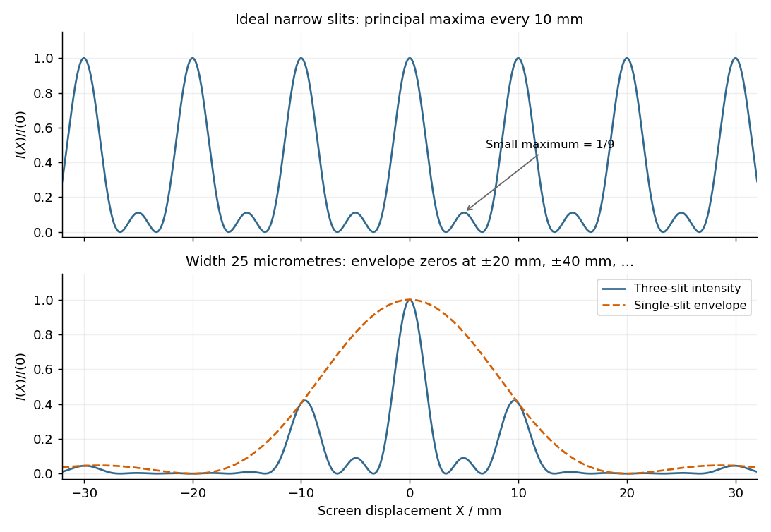
Original calculated Fraunhofer diffraction patterns for three narrow slits and for three finite-width slits
. Details. 
For a fixed transverse normal mode, define its cutoff angular frequencyThe longitudinal phase velocity and group velocity, for propagation in , areThus , and . The large longitudinal phase velocity reflects the geometry of the transverse standing wave and does not imply faster transport of energy than the membrane wave speed.
The cutoff frequency of a membrane waveguide for mode isAt cutoff and ; the longitudinal phase velocity has no finite value. Below cutoff,and a bounded field excited at decays as . It is an evanescent wave, rather than a freely propagating mode carrying net time-averaged energy flux down an indefinitely long uniform strip. A finite section can still transmit through coupling of evanescent fields.
Twice differentiating the proposed normal mode givesIt therefore solves the two-dimensional wave equation precisely whenThe fixed-edge boundary conditions require . The first is automatic, and the second requires . The nonzero normal modes are thereforeThe apparent choice gives identically zero displacement for this sine solution. There are no imposed end conditions in , so is continuous rather than quantized by a second length. For a propagating mode it is real; the plus sign in the stated convention describes propagation in . Each positive integer labels a transverse standing wave across the strip.
There is no reflected wave when the characteristic mechanical impedances match:for the same tension. Then , and . If tensions were independently adjustable, the general condition would be , together with transverse-force matching; equality of densities alone would no longer be the universal criterion.
The reflected and transmitted mean-power fractions areFor strictly positive finite linear mass densities, ; a finite density step cannot produce exact total reflection. The ideal limits areThe first behaves as a fixed end; the second as a free end. In the free-end limit the transmitted displacement tends to , but its mechanical impedance tends to zero, so it carries vanishing power. Thus total reflected energy does not require a vanishing boundary displacement. “Entirely reflected” at a merely large density contrast is an approximation.
Place the join at , with an incident wave travelling from medium 1 towards medium 2. WriteContinuity of displacement and slope gives and . Hence reflection at a density step on a string givesFor , : the reflected transverse displacement has a phase reversal of . For , and there is no displacement-phase reversal. The transmitted displacement has no phase reversal for positive real mechanical impedances.
Ramsey frequency precision Created 2026-10-18 Updated 2026-10-25
The full width at half maximum of a fringe, the lifetime of quantum coherence, and the precision of an estimated frequency are different quantities. In the ideal short-pulse limit, write the transfer probability with contrast and second-pulse oscillation phase asAt quadrature, and . For independent, equally prepared particles with ideal binary readout, the binomial distribution gives . Local propagation of uncertainty therefore yields the displayed . For chosen , and , it is approximately , although the ideal fringe width is . This is an original counting-noise estimate at a known quadrature, not the accuracy of a historical clock or a guarantee of finding the correct fringe.
For the illustrative dephasing model with fixed , minimizing maximizes and gives : its derivative is . This conclusion changes if longer interrogation reduces the number of accepted particles or the repetition rate. Quantum decoherence, a distribution of flight times, reference oscillator noise and readout errors can reduce contrast; a fitted decay time need not identify one microscopic mechanism. More counting can improve precision while a reproducible cavity quantum phase offset still biases the frequency, as in atomic clock frequency shifts.
Past exam of the theoretical physics II course of the University of Cambridge 2019 4 e iii Solution 2026-10-18
The reduced density matrix has two eigenvalues equal to . Its Von Neumann entropy, which is the entanglement entropy of the bipartite pure state, isThis is one bit when base-two logarithms are used. It is the maximum entanglement entropy for a pair of two-dimensional systems, while the joint Von Neumann entropy of the singlet state remains zero.
Past exam of the theoretical physics II course of the University of Cambridge 2019 4 e ii Solution 2026-10-18
Taking the partial trace over the left atom in the singlet state gives the right-hand reduced density matrixThus every measurement on the right stream alone has the same statistics as B or C. The joint pure state is compatible with locally mixed states; the correlations reside in the full density operator.
There are unlisted articles, also show them or only show them.