
The equilibrium photon gas is isotropic, so the energy density per unit solid angle in a narrow angular-frequency interval is . For rays making angle with an outward surface normal, a surface element is crossed in time by rays initially in a volume . Only the outward hemisphere contributes. ThusThe hemispherical restriction supplies a factor and the directional projection supplies another . A small aperture in a cavity therefore emits this spectral power per unit area. A blackbody at the same temperature emits the same amount: otherwise radiation exchange between it and the aperture would violate thermal equilibrium.
Integrating Planck's law over all positive angular frequencies gives the total emitted heat flux densitySet . ThenThe remaining integral is independent of temperature, proving . Its value follows by expanding and integrating termwise:Consequently the Stefan–Boltzmann law isThis is emitted power alone. A body in a radiation environment also absorbs incoming radiation, which must be included when calculating net radiative cooling.
Each independent cavity mode is a quantum harmonic oscillator of angular frequency . Its occupation numbers represent the numbers of photons in that mode. At thermal equilibrium, photons can be absorbed and emitted by the walls, so their number is not conserved and the photon chemical potential is zero. The Boltzmann distribution of the oscillator excitations then givesThe expression supplied in the paper is the thermal excitation energy. The oscillator's temperature-independent zero-point energy is excluded from the emitted thermal radiation.
Putting and into the mode count from (a) gives the number of modes per unit cavity volume:Multiplying by the mean thermal energy in each mode yields Planck's law in the angular-frequency convention:The two photon polarizations are already included in the density of states; no further factor of two is needed. has units , whereas has units .
A cubic reflecting cavity supports standing waves with positive integer mode indices and wavevector components . A cell in mode space has volume . In the continuum approximation, a spherical shell of radius and thickness has one-eighth of its volume in the positive octant. There are two independent transverse photon polarizations for a generic wavevector. HenceThe photon energy is , so . ThereforeThis is the leading bulk density of states, valid when the cavity is large compared with the relevant wavelengths and many modes lie in the counting interval. A finite cavity has a discrete mode spectrum, with boundary corrections beyond this approximation. Modes with vanishing indices require separate boundary counting but do not change the leading term. Here is the reduced Planck constant, as printed in the original PDF; replacing it by would introduce an erroneous factor of .
For a diatomic ideal gas in the usual regime with three translational and two rotational quadratic degrees of freedom, but frozen vibrational excitation, the equipartition theorem givesThe Brayton cycle efficiency is thereforeThe constant-pressure expansion has , while the compression has . The same relations give . Thus, in units of the minimum temperature,The maximum and minimum temperatures are and . A Carnot cycle between those extremes hasThe difference is about percentage points. In the Brayton cycle, heat is supplied and rejected over ranges of temperature; the whole input is not supplied at , nor is the whole rejection made at . This explains the lower efficiency even for mechanically ideal stages. Absolute state temperatures are not supplied, so is an explicit standard diatomic-gas approximation rather than a conclusion about all possible rotational and vibrational excitation regimes.
This is the Brayton cycle. Assume fixed gas amount, constant heat capacities, and internally reversible adiabatic processes, as intended by the ideal engine model. Put andCombining with the ideal gas law gives along either reversible ideal-gas adiabat. ThereforeDuring a constant-pressure process the heat supplied equals the enthalpy increase. If is the molar heat capacity at constant pressure, the positive heat input and output areThe insulated branches exchange no heat, so the first law of thermodynamics gives . HenceAn adiabatic process alone need not be an isentropic process; the relations used here also require internal reversibility. Dissipative compression or expansion would require extra information and would not, in general, obey this efficiency formula.
For the numbered engine, denote the low and high pressures by and . Let denote the molar gas constant. The ideal gas law makes the constant-pressure branches straight rays in a temperature-volume diagram:The high-pressure ray is steeper. For a constant heat capacity ratio , each reversible ideal-gas adiabat obeysConsequently curves upward and left during compression; goes upward and right along the steeper ray; curves downward and right during expansion; and goes downward and left along the shallower ray.
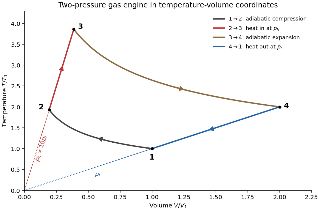
The plot is an original calculation for , and ; its state directions follow the original paper. The dashed extensions identify the two constant-pressure rays, not additional stages of the cycle.
The complete cycle must be a reversible thermodynamic process: no friction, viscous dissipation, unrestrained expansion, or other source of entropy. Each moving boundary must be arbitrarily close to mechanical equilibrium. Heat transfer to or from a bath must occur across an infinitesimal temperature difference, and the insulated stages must be genuinely adiabatic processes. There must also be no direct heat leak between the heat baths.
For an engine exchanging heat only with these two heat baths, the Second law of thermodynamics givesand thusPractical engines generate entropy through finite temperature differences, friction and other dissipative effects. They therefore fall below the Carnot cycle limit. Approaching reversible heat exchange generally requires vanishingly slow operation for a finite heat-transfer apparatus, limiting useful power.
Because the working substance returns to its original thermodynamic state, its net entropy change is zero. There is no entropy change on either reversible ideal-gas adiabat; on each isothermal process the entropy transfer is the exchanged heat divided by the bath's absolute temperature. HenceThe first law of thermodynamics over a complete cycle gives . The thermal efficiency is thereforeThe use of kelvins is essential. This result does not depend on the working substance. For the ideal gas illustration, the two reversible ideal-gas adiabats imply , so ; the explicit heat expressions in (a) give the same ratio.
Use an ideal gas to illustrate the Carnot cycle, with hot and cold heat baths at and . The four processes are all reversible thermodynamic processes. Lettered states below belong only to this illustration; the engine later in the question uses numbered states.
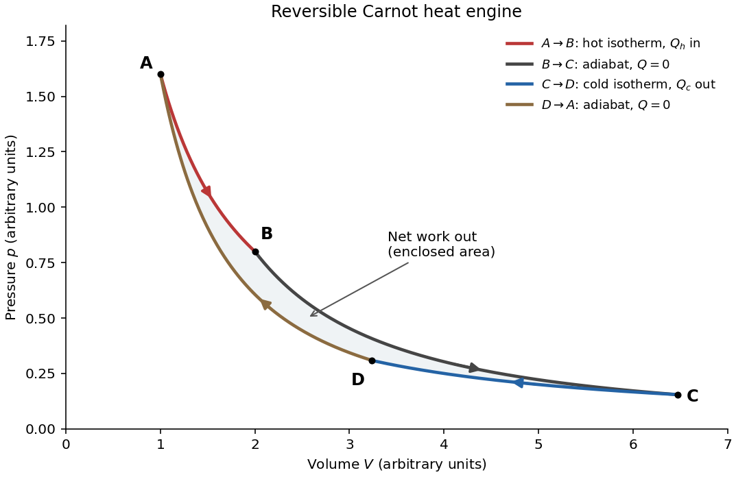


Starting at , perform the following four stages:
- : isothermal expansion at . The gas absorbs heat from the hot heat bath and does work. Its internal energy is unchanged, so .
- : reversible ideal-gas adiabat during expansion. Insulation prevents heat transfer; work done by the gas reduces its internal energy and lowers its temperature from to .
- : isothermal compression at . Work done on the gas is rejected as heat to the cold heat bath, with .
- : insulated adiabatic compression, performed reversibly, raises the temperature back to and closes the cycle.
An incident electromagnetic wave generally produces reflected and transmitted waves because the two media have different electromagnetic response. Consider a flat interface between homogeneous, linear, lossless media with permittivities and magnetic permeabilities . Their wave speeds and wave impedances areFor each plane electromagnetic wave, . With no free surface charge or current, the interface conditions for electromagnetic fields require continuous tangential and normal . Equality of the phase at every point on the boundary gives equal angular frequencies and tangential wavevectors. Hence the reflection angle equals the incidence angle and Snell's law iswhere and each angle is measured from the normal.
At normal incidence use the same tangential axis for all electric amplitudes. The two independent boundary equations areSolving gives the amplitude Fresnel equationsFor nonmagnetic media, these become and . Reflection into a medium of larger refractive index therefore reverses the electric amplitude's sign at normal incidence.
The normal Poynting vector determines the reflected and transmitted fractions of incident power. At normal incidence,It is the power fractions, rather than the squared electric amplitudes alone, that add to unity.
At oblique incidence separate transverse electric polarization (, electric field perpendicular to the incidence plane) from transverse magnetic polarization (, electric field in that plane). For nonmagnetic media, writing and , the Fresnel equations areHere choose a common direction and, for each ray, the direction as . This makes the reflected basis reverse its tangential direction at normal incidence, explaining why the displayed then has the opposite sign to . Physical reflectance is independent of this sign convention. For either polarization with propagating transmission,For polarization, zero reflection occurs at the Brewster angle . If , incidence above the critical angle for total internal reflection produces an evanescent field in total internal reflection and for an isolated lossless interface. A lossy second medium requires complex response coefficients and an absorption term in the energy balance.
Because the magnetic field obeys , it can be represented locally as the curl of a magnetic vector potential:This automatically enforces the absence of magnetic monopoles. It is also a global representation throughout ordinary all-space problems without monopole singularities. It is not unique: the gauge transformationleaves unchanged because the curl of a gradient vanishes. In a time-dependent problem,makes the same transformation leave both physical fields unchanged and automatically satisfies Faraday's law.
In vacuum magnetostatics, choose the Coulomb gauge . Substitution into Ampère's law and the identity givesfor a localized steady electric current density and a potential vanishing at infinity. Taking the curl recovers the Biot-Savart law. The magnetic vector potential converts a constrained vector field problem into componentwise Poisson equations once a gauge is chosen.
For a uniform magnetic field, is a convenient choice. For a localized magnetic dipole moment , the leading far-field potential isAnother useful relation is Stokes theorem, which relates a closed-path integral to the magnetic flux through a spanning surface:The units of are , equivalently .
An electrical insulator has no freely conducting bulk charge in the ideal static description, but an applied electric field can displace bound positive and negative charge relative to one another. The resulting electric dipole moments per unit volume define the polarization density . Distortion of electronic charge clouds, relative displacement of ions, and partial alignment of permanent molecular electric dipoles can all contribute. Thermal agitation opposes the last mechanism.
For a weak field in a linear isotropic dielectric, the constitutive law isHere is the electric susceptibility, is the permittivity, and is the electric displacement field. In an anisotropic material, is a tensor and need not be parallel to . These response laws describe the macroscopic field, not necessarily the microscopic field acting on one molecule.
Spatial variation and surface termination of the polarization density give bound charge and bound current through the bound charge densitieswhere is outward from the material. Thus uniform polarization density has no bulk bound charge, but generally has opposite bound charges on opposing surfaces. Gauss's law can be rewritten asWith no free surface charge, the normal component of is continuous across an interface; the tangential electric field is continuous in electrostatics.
For example, fill a parallel-plate capacitor of plate area and gap with a uniform dielectric, neglecting fringing. At fixed free plate charge , , soThe induced bound surface charges oppose the original field, reducing the electric field and potential difference at fixed . At fixed applied potential difference, the field remains and the battery instead supplies more free charge. The electric displacement field separates these free-charge and bound-charge roles.
The method of images solves certain electrostatics problems by replacing a conductor by fictitious electric charges outside the region where the solution is required. The replacement must satisfy the actual boundary values of the electric potential as well as the prescribed sources. The uniqueness of Poisson equation then establishes that the constructed electric potential equals the physical one in that region. The image locations are mathematical devices; they are not real charges inside the metal.
For a point charge at above an infinite grounded conducting plane , put an image charge at . In a cylindrical coordinate system with coordinates the potential in the physical region isThis vanishes at , has the required singularity at the real charge, and tends to zero at infinity. With electric field , the induced surface charge density follows from the normal field immediately above the conductor:The force on is the field of the image evaluated at the real charge:The electrostatic energy relative to infinite separation is . The factor accounts for the fact that the induced charge changes as the real charge is assembled; treating the image as an independently fixed physical charge would give the wrong energy.
A second standard geometry is a grounded conducting sphere of radius with a charge a distance from its centre. Its exterior field is generated by an image at distance from the centre on the line towards the real charge. On the sphere the distances to the real and image charges are in the ratio , making their potentials cancel. For an isolated neutral sphere, an additional central image makes the total induced charge zero and leaves the surface an equipotential. The construction is powerful for suitable symmetric boundaries, but arbitrary boundaries do not in general admit a finite image system.
Set . Comparing with the untapered expression in part (d), using the same and large radius ,The stated limit makes , soThe taper concentrates magnetic flux into a smaller pole-face area, increasing the gap magnetic field intensity and magnetic flux density for the same winding electric current. If , the enhancement approaches . If instead , the gap dominates the magnetic reluctance and the enhancement approaches unity: both fields approach .
The benefit is therefore strongest when the untapered core's contribution is significant, while the taper lengths contribute little. The same-core-length convention is the comparison defined by parts (d) and (e); if one instead fixes the full iron path length, the untapered comparator has length , a difference negligible in the stated limit. A smaller gap area can increase the field even though the total magnetic flux need not increase. Magnetic saturation and magnetic fringing, excluded from this model, limit the ideal concentration.
Let the approximately conserved magnetic flux be . ThenThe length shown in the original diagram is the untapered core arc; the two tapers are separate lengths each. In the untapered core, flux conservation givesFor one taper use distance from its narrow end. The straight taper in the diagram has local radiusand magnetic field intensityIts contribution to the line integral in the magnetostatic Ampère law is found explicitly:Adding the gap, the untapered arc and both tapers givesThereforeThis uses a linear radius profile, approximately uniform magnetic flux density over each section, a linear constant magnetic permeability, and negligible leakage and magnetic fringing. For a non-linear taper profile the honest generalization isThus an arbitrary smooth taper with the same end radii and length need not give the printed formula; the straight-sided geometry supplies the additional information.
With uniform section and negligible magnetic fringing, constant magnetic flux gives equal magnetic flux densities in the core and gap:Here is the core arc length and the additional gap length. Applying the magnetostatic Ampère law around the complete magnetic circuit,Consequently,This tends to when the gap dominates the magnetic reluctance, , and reduces to the no-gap result as . The gap magnetic flux density is .
For the closed untapered torus, apply the magnetostatic Ampère law to a circular path through the core. It links all turns, each carrying electric current :Since , variation of the path length and of the tangential magnetic field intensity across the section is negligible. Thus , giving, within this thin-torus approximation,The units are . The core magnetic flux density is in the linear material model.
The starting point is Gauss's law for magnetism, : a flux tube carries the same magnetic flux through successive transverse sections. To identify that tube approximately with the physical core, one must also make a negligible-leakage approximation. The large core magnetic permeability makes the core route much less reluctant than competing paths through the surrounding air; the small gap further reduces the incentive for a long external return path. The gentle taper, , lets the field follow the changing section with only small transverse corrections.
For two cuts and the intervening lateral surface, the divergence theorem gives . Neglecting lateral leakage givesThe normal magnetic flux density is continuous at each core–air interface by part (a), so this same magnetic flux crosses the gap. To use the gap's geometrical area in the later formulas, the magnetic fringing must also be negligible, normally requiring . This is the small-gap interpretation of the paper's approximation. Large magnetic permeability alone does not eliminate leakage or magnetic fringing for arbitrary gap geometry.
Let the unit normal point from material 1 to material 2, and let their relative magnetic permeabilities be , so for linear isotropic media. Apply Gauss's law for magnetism to an infinitesimal Gaussian pillbox straddling the interface. The side contribution vanishes as its height tends to zero, leavingThe normal magnetic flux density is continuous.
Next use a narrow rectangular Amperian loop crossing the interface. The two short-side contributions vanish in the zero-height limit. The magnetostatic Ampère law for magnetic field intensity giveswhere is any free surface current density. Thus, if there is no free surface current density on the interface, the tangential magnetic field intensity is continuous. In that case the component relations areThe distinction between free and bound electric currents matters: bound currents due to magnetization are already incorporated in the definition of magnetic field intensity. A change of magnetic permeability alone does not make the tangential magnetic flux density continuous.
On the curved wire surface, the outward normal is and the Poynting vector has the constant radial value . Its outward flux isThe Poynting vector is radial, so it has zero normal component on the two end faces in this approximation. This is therefore also the outward flux through the complete wire surface. Equivalently, positive electromagnetic power flows inward.
The fields are steady, so the stored electromagnetic energy does not change. Poynting's theorem consequently requires the incoming power to equal the Ohmic heating in part (e), exactly as found. The energy reaches the wire through the surrounding electromagnetic field. A local check is .
There are unlisted articles, also show them or only show them.