
Past exam of the theoretical physics II course of the University of Cambridge 2018 2 e Solution 2026-10-18
The delta-shell Born amplitude is first order in the potential strength:It retains finite-energy angular dependence and includes the leading weak-coupling contributions of all partial waves. By contrast, the supplied is the zero-energy limit of the exact S-wave scattering amplitude. It is isotropic, depends nonlinearly on , and captures the scattering-length pole missed by first-order perturbation theory.
At finite energy the exact S-wave amplitude is insteadwhich is generally complex and obeys elastic unitarity. Its zero-energy limit is for finite scattering length. Thus the two expressions printed in the question represent different approximations; the energy-independent S-wave expression is not the full finite- result of part (c).
Their common regime requires both weak coupling and low energy:Then , soConsequentlyin that joint regime. Low energy alone does not remove the nonperturbative denominator , while weak coupling alone does not remove higher-partial-wave angular dependence.
Past exam of the theoretical physics II course of the University of Cambridge 2018 2 d Solution 2026-10-18
The scattering length is . Since and , the exact phase shift gives, away from the pole,Thus plot against , so that both axes are dimensionless.
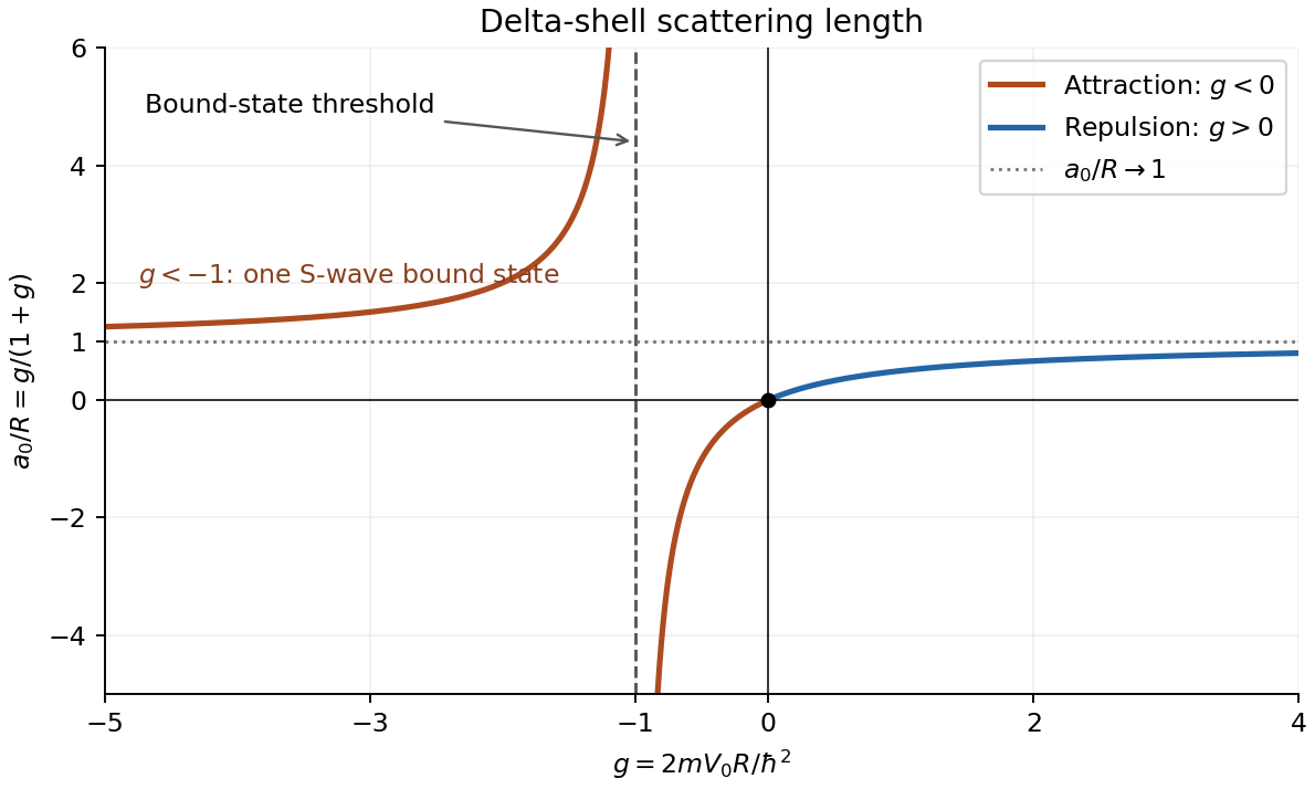
Delta-shell scattering length versus dimensionless coupling, with the bound-state threshold at g = −1
. Details. 
For repulsion, , the curve rises from zero to the horizontal asymptote , staying between zero and one. For weak attraction, , the scattering length is negative and tends to as . For stronger attraction, , it is positive and greater than , tending to as and to as . Its only zero is .
The pole at is the zero-energy threshold of an S-wave bound state. To see this directly, use inside and outside for energy . The same derivative jump givesThis approaches as and admits a positive for . At the threshold the scattering length diverges; this is a zero-energy scattering resonance, not a divergence of the finite-energy cross-section beyond its partial-wave unitarity bound. These are the main features of the scattering length of a delta-shell potential.
Past exam of the theoretical physics II course of the University of Cambridge 2018 2 c Solution 2026-10-18
Away from the shell, the reduced radial equation is free. Regularity at the origin and the definition of the S-wave phase shift giveThe reduced radial wave function is continuous at ; otherwise its second derivative would contain a delta derivative not present in the equation. Integrating the equation across the shell gives the jumpDivide by the common shell value and substitute the two free solutions. This yieldsIf the shell value vanishes, use the undivided matching equations or a continuous limit rather than this logarithmic-derivative division. For an explicit phase shift of a delta-shell potential, write and . The cotangent addition formula givesThe phase is defined modulo ; choose its branch continuously as energy or coupling varies. At zero coupling the physical phase shift is zero.
Past exam of the theoretical physics II course of the University of Cambridge 2018 2 b Solution 2026-10-18
In the first Born approximation, with incident and outgoing wave vectors , put . For elastic scattering,Choose the polar axis along . The angular integral isThe radial Dirac delta distribution then givesThus, introducing the dimensionless shell strength ,The forward value is the continuous limit . This is the delta-shell Born amplitude, with its angular dependence expressed through the momentum transfer.
Past exam of the theoretical physics II course of the University of Cambridge 2018 2 a Solution 2026-10-18
For a short-range potential, an incident plane wave of unit amplitude and wave vector has the large-distance scattering wavefunctionThe coefficient is the scattering amplitude. For a central potential it depends only on the scattering angle . The incident probability current is , while the scattered radial current is to leading order. Their ratio givesThese are the differential scattering cross-section and total cross section for elastic scattering with the same incident and outgoing wave number.
The expression is asymptotic: it specifies the outgoing wave's leading term, not its finite-distance radial corrections or its form inside the interaction region. In particular, for angle-dependent , the spherical term by itself has an angular-Laplacian contribution of order to the free wave equation, which is cancelled by subleading terms in the exact solution.
Past exam of the theoretical physics II course of the University of Cambridge 2018 1 e Solution 2026-10-18
The occupation formula from part (b) givesConsequentlyThe independent occupation numbers are each zero or one. The Hamiltonian is independent of , so its four states haveEach energy admits or ; these states differ by occupancy of the zero-energy mode. The ground energy is for either sign of . These degeneracies refer to the full two-mode fermionic Fock space. If one separately restricts to a fixed global fermion parity, only one state at each energy remains in that parity sector.
Past exam of the theoretical physics II course of the University of Cambridge 2018 1 d Solution 2026-10-18
For any two distinct normalized Majorana fermion operators , let . ThenandThe same applies to . Both specified pairs have this form. Moreover, the Majorana operators entering are all distinct from those entering , so every cross anticommutator is zero. ThereforeThus are ordinary fermionic annihilation operators, constructed by a different pairing of the four Majorana operators.
Past exam of the theoretical physics II course of the University of Cambridge 2018 1 c Solution 2026-10-18
Use and . Moving operators from different modes past one another introduces a minus sign. Direct expansion givesThus, for real hopping and pairing parameters,At this becomesUse for time to distinguish it from the hopping amplitude . Each unused Majorana operator anticommutes with both factors in , so commuting it through their product gives two minus signs. Hence . The Heisenberg picture equation therefore givesThese are the two uncoupled Majorana zero modes.
Past exam of the theoretical physics II course of the University of Cambridge 2018 1 b Solution 2026-10-18
Expand the anticommutators using the relations in part (a). The terms with two creation or two annihilation operators vanish, leavingEach Majorana fermion operator is Hermitian and squares to the identity. In particular, , so this expression cannot distinguish an empty mode from an occupied one. A single Majorana operator is its own adjoint and does not supply distinct creation and annihilation operators for such an occupation.
An occupation can instead be assigned after pairing Majorana operators into a fermionic mode. For two distinct Majorana operators ,This is a nontrivial projection operator with eigenvalues zero and one. Thus occupation belongs to a chosen pair of Majorana operators, not to an individual Majorana operator.
Past exam of the theoretical physics II course of the University of Cambridge 2018 1 a Solution 2026-10-18
For independent bosonic modes, the canonical commutation relation isFor independent fermionic modes, the canonical anticommutation relations arewhere and . The creation operator is the adjoint of the annihilation operator. In either case the mode's number operator iswith or as appropriate. It measures the mode's occupation number. Its possible eigenvalues areFor fermions, implies , so the number operator is a projection. This expresses the exclusion of double occupation of one fermionic mode. The total particle number is .
Past exam of the theoretical physics II course of the University of Cambridge 2017 4 e Solution 2026-10-18
Let and for , as required by the cosine form of the Jacobi-Anger expansion. For a central real potential, the Partial-wave S-matrix is . Splitting each shifted radial cosine into incoming and outgoing exponentials leaves its incoming coefficient unchanged and multiplies its outgoing coefficient by . Subtracting the incident plane wave givesComparing with the prescribed scattering amplitude convention yields the two-dimensional partial-wave scattering formula,Orthogonality gives and for , while all cross terms vanish. HenceThe multiplicities printed in this part are reversed. With those printed values and every , the purported free wave would be , rather than the required incident plane wave. The extra contains an incoming cylindrical wave, which cannot be absorbed into . The formulas above use the corrected multiplicities and therefore satisfy the specified scattering boundary condition.
Past exam of the theoretical physics II course of the University of Cambridge 2017 4 d Solution 2026-10-18
For , expand . The lowest power producing the Fourier harmonic is . Meanwhile . Matching these lowest powers gives .
For negative order use and the equality of the positive and negative Fourier coefficients of this even function of . This gives . Therefore the Jacobi-Anger expansion isThe cosine form has multiplicity one for and two for every positive . Those multiplicities are essential for matching the incident plane wave.
Past exam of the theoretical physics II course of the University of Cambridge 2017 4 c Solution 2026-10-18
The incident plane wave is periodic in , so expand it as a Fourier series . Substitution into the Helmholtz equation, with , gives the radial Bessel differential equationRegularity at the origin selects the Bessel function of the first kind, rather than the singular second solution. ThusThe coefficients are independent of ; their values follow from matching near the origin in the next part. The completed identity is the Jacobi-Anger expansion.
Past exam of the theoretical physics II course of the University of Cambridge 2017 4 b Solution 2026-10-18
The incident plane wave carries probability current . For the separated outgoing wave from the previous part,The rate through a distant arc is . Dividing by incident flux defines the differential two-dimensional scattering cross-section,Because is dimensionless, has units of length, as appropriate for scattering in a plane.
Past exam of the theoretical physics II course of the University of Cambridge 2017 4 a Solution 2026-10-18
Outside a short-range scattering region, the stationary Schrödinger equation reduces to the two-dimensional Helmholtz equation. Separation in polar coordinates gives outgoing radial Hankel functions, whose large- dependence is . The same power follows from conserved probability current: a circle has length proportional to , so the squared outgoing amplitude must decrease as .
For an incident plane wave in the direction, adopt the dimensionless amplitude conventionThe phase and factor specify the definition of ; they can be absorbed into a differently normalized scattering amplitude. Here they are kept exactly so that the later two-dimensional scattering cross-section follows consistently.
Past exam of the theoretical physics II course of the University of Cambridge 2017 3 e Solution 2026-10-18
For fixed , write . The bound contribution to the quantum propagator of an attractive delta potential remains . For its continuum, the stationary phase is at , where . The Gaussian oscillatory integral and its derivative giveConsequentlyThe continuum decays as , but the full kernel has a persistent oscillating bound state contribution and no ordinary complex limit. This expansion requires ; it is not uniform in the zero-coupling limit, where the bound state disappears and the free kernel instead decays as .
Past exam of the theoretical physics II course of the University of Cambridge 2017 3 d Solution 2026-10-18
At the origin, the normalized bound state in a delta potential contributes , and the odd scattering eigenfunctions contribute zero. The even continuum functions from the preceding part haveTheir energy is . Inserting these weights into the spectral resolution of a quantum propagator, and using evenness to extend the integral to the whole real axis, yields for This is the quantum propagator of an attractive delta potential. The printed continuum exponent has an extra factor of : its time phase must be . This correction also makes the exponent dimensionless. Oscillatory integrals are understood with an infinitesimal positive convergence factor before taking its limit.
Past exam of the theoretical physics II course of the University of Cambridge 2017 3 c Solution 2026-10-18
Choose the even-channel scattering phase shift convention for . The delta potential derivative jump givesso, choosing the branch that tends to zero as ,An odd scattering eigenfunction is : it vanishes at the interaction and its derivative is continuous, so it acquires no scattering phase shift. These parity channels, with the bound state, give the continuum part of the spectral resolution of a quantum propagator.
Past exam of the theoretical physics II course of the University of Cambridge 2017 3 b Solution 2026-10-18
Away from the delta potential, the decaying bound state obeys . Integrating the Schrödinger equation across the attractive interaction givesFor an even exponential, the left side is . ThereforeThe normalized bound state in a delta potential is , since . The single positive solution for gives one bound state; an odd decaying wave cannot be both continuous and nonzero with this interaction.
Past exam of the theoretical physics II course of the University of Cambridge 2017 3 a Solution 2026-10-18
For a time-independent Hamiltonian operator, the time-evolution operator is , with . Insert its resolution of identity in normalized energy eigenstates:Since , the retarded quantum propagator in the question isThe Heaviside step function imposes the chosen retarded convention. If the Hamiltonian operator has a continuous spectrum, the spectral sum includes its continuum integral; it must not be restricted to bound states. The spectral resolution of a quantum propagator also shows that tends to as . With the step factor it obeys ; the corresponding Green function with a unit delta source is .
There are unlisted articles, also show them or only show them.