
The four direct beta decay branching fractions exhaust the parent decays in the model, soHere the question's are dimensionless branching fractions, despite the conventional use of for a dimensionful decay width. Its “zeroth excited state” means the daughter ground state. Cascades through an excited level do not count as an additional direct beta branch to it.
Retain as defined in Case 1. In the laboratory, A moves and B is stationary. Transform A's fields and add B's unchanged electrostatic field:The laboratory linear charge densities are and , with electric currents and .
In , A is stationary while B moves with velocity . Thus A contributes its rest electrostatic field, and B contributes the boosted electric field and the opposite-sign convective magnetic field:The densities in this frame are , , with and . Substituting the laboratory result into part (a) gives the same fields; for instance . The magnetic contribution attributed to A disappears in its own frame, but B's contribution does not.
Write , , and , evaluated at the same transverse coordinates . A superscript labels each filament's own rest frame, rather than a single common frame in all cases. The filaments are infinite and uniform along , so the change of longitudinal coordinate under a Lorentz boost creates no extra dependence in these functions. After the acceleration transients have passed, the magnetic field of each filament vanishes in its own rest frame.
For a filament moving at , use the inverse of part (a): its transverse electric field in the laboratory is and its magnetic field is . Superposition for the two co-moving filaments therefore gives, in ,In the common co-moving frame both filaments are at rest, soFor example, , a useful sign check. The supplied is the proper linear charge density. Thus each laboratory density is and each laboratory electric current is , consistently with length contraction and the four-current transformation. In each density is and both currents vanish.
Keep source, observer and magnetic field in their original places, but interchange the physical polarizers, including their pass-axis orientations. The forward order is then , glass, , so the new Jones matrix is again . ConsequentlyThis is the same intensity change as exchanging source and observer. At the field that maximizes the original forward transmission, the swapped arrangement blocks the beam. If both operations were performed together, the original order relative to propagation would be restored and so would the original transmission. The answer concerns exchanging the two differently oriented pass axes; simply relabelling two identical polarizers while leaving their axes fixed would not change the apparatus.
Keep the magnetic field fixed in the laboratory and exchange source and observer. The incident unpolarized light now meets first. In fixed transverse laboratory axes the backward glass map is still , not : this is optical nonreciprocity of the Faraday effect. The order of the two polarizers is reversed, soThe reverse light intensity is thereforeFor the optimal forward setting , it vanishes: the input selected by rotates to and is blocked by . At a general field, . The result assumes equal incident light intensities in the two experiments. Treating the glass as a reciprocal natural optical rotator would predict cancellation of its laboratory rotation on reversal and would give the wrong answer here.
The lower derivative index and the upper electromagnetic four-potential index are fully contracted. For a constant Lorentz transformation,HenceThis is a statement about Lorentz transformations, not electromagnetic gauge transformations. The quantity is not generally gauge invariant; setting it to zero is the Lorenz gauge condition, which is Lorentz covariant because zero remains zero in every inertial frame.
The chain rule givesThusDifferentiation with respect to a contravariant coordinate has a lower transformation index. In inertial Cartesian coordinates in Minkowski spacetime, no connection term is needed for this coordinate transformation of a derivative acting on a scalar; Lorentz transformations have constant Jacobians.
First lower the index of the four-current with the Minkowski metric: . The displayed expression is thenThereforeIts one free lower index transforms with the inverse coordinate Jacobian. The contraction with the metric here lowers an index; it does not make the current a scalar because the index remains free.
The upper index identifies as a contravariant Lorentz four-vector, obeying the rank-one contravariant tensor transformation law. Its components transform with the coordinate Jacobian,It is not invariant component by component. Its contracted square , for metric signature , is a Lorentz invariant. This distinguishes a contravariant transformation law from an invariant scalar.
Velocity-averaged Ramsey line 2026-10-18
Let each drive region have length and the drive-free gap have length , measured edge to edge. A particle of constant speed experiences and . For a normalized detected-beam speed probability density function , sum the transition probabilities, not the probability amplitudes of different particles:The displayed is an ideal effusion flux distribution, with speed scale , uniform transmission and speed-independent detection efficiency. It is not a claim about any particular clock's selected beam. The substitution gives , proving normalization. Actual apertures, state selection and readout can change the effective weights.
For an original example choose , , and . The reference particle has , and resonant pulses. The instantaneous-pulse width would be . The exact finite-pulse width for that single speed is about ; the chosen distribution also reduces the on-resonance average to approximately because not every particle receives a pulse.
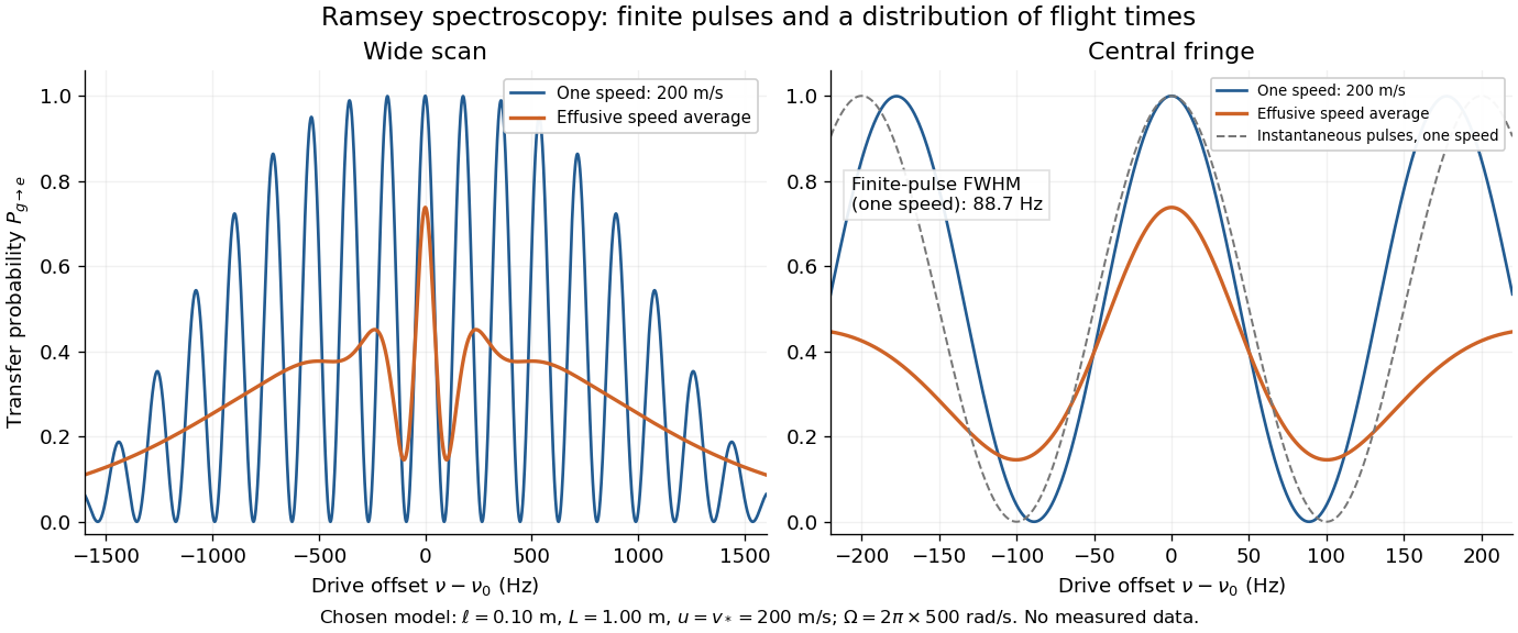

Different velocities smear side fringes because varies across the beam. Nevertheless every term is even in , so this symmetric ideal-model average has no odd line asymmetry that could displace the central lock point. Reduced contrast or altered width alone is not evidence of a shifted line center. A speed-dependent transition shift or unequal drive quantum phases changes that conclusion; atomic clock frequency shifts explains why these distinctions matter experimentally.
Finite-pulse Ramsey phase response 2026-10-18
Keep the first pulse's oscillation phase zero and give the second phase in the Driven two-level Rabi model. Its upper off-diagonal Hamiltonian operator entry is . Multiplying the two pulse unitary operators and the free-flight unitary operator givesThe Born rule gives the displayed phase-dependent form using the of the Ramsey fringe envelope. Thus reproduces the existing expression, while turns a resonant transfer maximum into zero transfer. A single pulse's population is insensitive to its drive phase; the second coherent interaction makes their difference observable. An uncontrolled, uniformly random instead averages this probability to , leaving the broad pulse response but removing the dark-flight fringes.
Finite pulses also contribute to the near-resonant frequency slope. For , differentiating at gives . Consequently the phase near resonance isAt the exact resonant slope is . For the plotted parameters ; the near-resonant estimate explains why the exact finite-pulse width below differs from . The slope is exact at resonance under these assumptions, while this width estimate uses the local phase expansion. A velocity distribution requires averaging the full response, not substituting one effective flight time.
Ramsey fringe envelope 2026-10-18
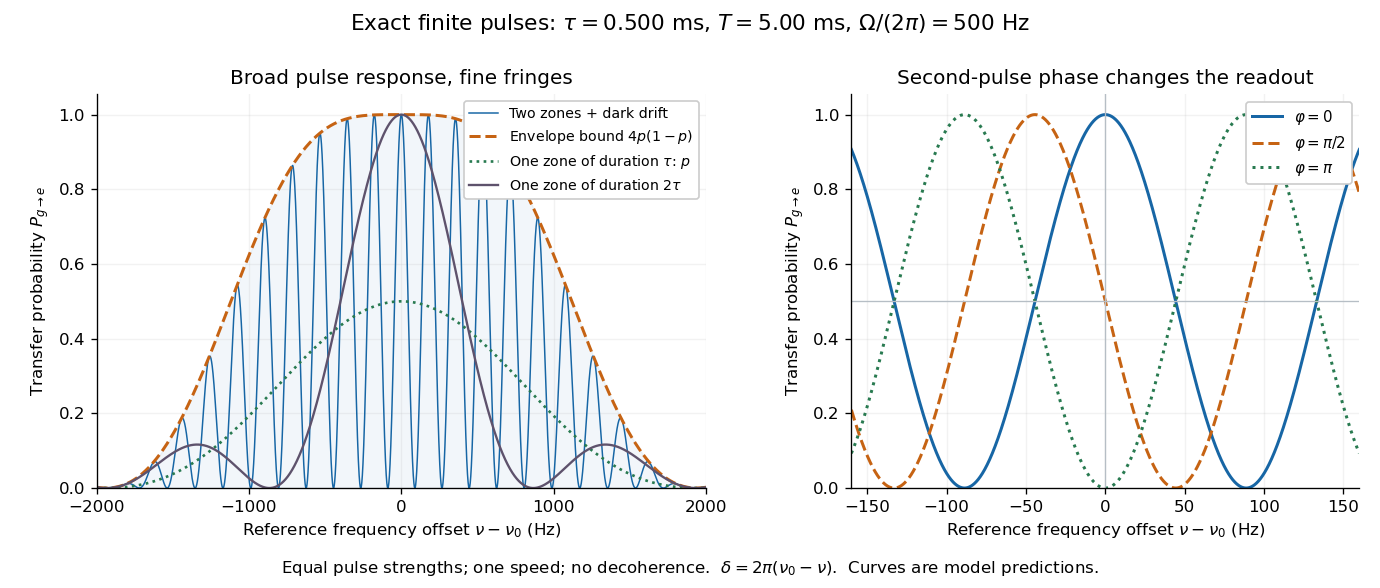
The exact finite-pulse Ramsey transition probability separates a slowly varying pulse response from rapid quantum interference. Define the single-zone transfer probability and a pulse-induced quantum phase bySince , factorizing the real bracket in the original formula givesWhere , the probability is zero and need not be defined. Elsewhere this identity proves the envelope bound without a weak-drive assumption. The envelope is not the single-zone response : two equal coherent interactions have different transfer weights. A contiguous resonant Rabi pi pulse of duration provides another useful comparison with the same total drive duration, but no dark interval. Its line is broad because it has no long flight phase.

Finite-pulse Ramsey transition probability 2026-10-18
Use the Driven two-level Rabi model in the ordered basis , with Pauli matrices satisfying . Let the Rabi detuning be , in angular frequency, while and are ordinary frequencies in hertz. Assume two identical square pulses, equal drive oscillation phases, constant positive Rabi angular frequency , constant during pulses and flight, and no quantum decoherence or loss. The rotating-wave approximation and isolation of the chosen two-level system are required, just as for the Driven two-level Rabi model. Free flight means no transverse drive; the reference oscillator continues running.
The pulse and free-flight Hamiltonian operators in the rotating frame areThe Pauli matrix multiplication law gives . Thus the exact special unitary group pulse matrix for this effective Hamiltonian operator, and the flight matrix, areThe sequence is . Starting in , matrix multiplication and the Born rule giveThis retains the tilted rotation axis and quantum phase accumulated during each finite pulse. At resonance it gives ; with no flight it reduces to the single square-pulse response for duration . Both checks would fail if arbitrary ideal rotations were silently substituted at nonzero Rabi detuning.
For resonant pulse area , and , the central fringe approachesIts half-height points are , so the central peak's full width at half maximum is in hertz, or in angular frequency. This width assumes an effectively flat pulse envelope across that central peak, one flight time and unit contrast; it is neither a universal finite-pulse width nor a frequency uncertainty. Longer flight lets a smaller frequency difference accumulate the same observable quantum phase.
The two pulses here have the same sign and the plotted outcome is transfer to . The earlier Ramsey interferometry example uses an inverse analysis pulse and reports return to its initial label. Specifying the measured outcome and pulse oscillation phases reconciles the two conventions. In a beam the lengths and speed determine and ; in the Quantronium Ramsey interference experiment electronics set the pulse times for a stationary circuit.
Ramsey spectroscopy 2026-10-18
Ramsey spectroscopy measures a transition frequency by comparing the relative quantum phase acquired between two coherent interactions with the reference oscillator. In a beam, a state selector and apertures admit particular internal quantum states and trajectories; an analyzer and detector measure state-dependent transmission. In an optically prepared atomic clock, optical pumping and fluorescence can perform those functions. The preparation and readout determine which part of the beam contributes; they are not themselves the two coherent interactions.
For an ideal accepted particle, the first resonant half-duration Rabi pi pulse splits the probability amplitude between and . The second combines two indistinguishable alternatives: a transition in the first region followed by no transition in the second, or the reverse. Their relative quantum phase depends on the dark flight and the drive oscillation phases. Adding probability amplitudes gives quantum interference; adding only the two alternatives' probabilities would erase the fringe. “Dark” means that the transverse drive is absent: a static magnetic field and the internal Hamiltonian operator can still act.
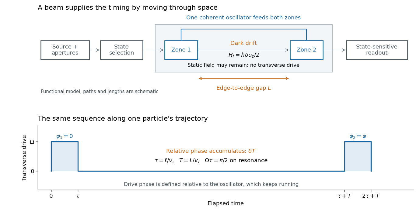

The useful separation is between pulse duration and phase-accumulation time. Short regions can share one coherent oscillator while a long drive-free interval resolves small frequency differences. A scan over reference frequency locates a fringe pattern; controlled changes of the second pulse's oscillation phase distinguish that coherent signal from phase-insensitive background. A reference scan must also identify the central fringe before atomic clock frequency lock, because neighboring fringes provide competing lock points.
For the infinite system with outward drift, total probability remains one, but probability at a fixed distance from the root eventually decreases as the walker moves away. The question concerns this local decay, not a loss of total probability.
The independent dimensions of the continuum coefficients are and . The drift-diffusion decay time and its associated length are, up to numerical factors:Equivalently, equating the drift distance to the diffusive width of order gives this crossover scale. Rescaling and removes the dimensional coefficients from the equation.
With the conventional coefficients used in the requested continuum derivation,where the last expression suppresses the numerical factor as requested. The elementary drifted Gaussian distribution on the full line hasAt fixed , its exponential decay factor is , so an exponential e-folding time would conventionally be called , consistent with the same dimensional scale. The reflecting half-line changes the spatial form and algebraic prefactor. The substitution gives , displaying the same exponential scale for outward drift.
For , and no finite drift-induced exponential decay time exists: the probability near the root decays only algebraically. For the finite-bias, deterministic-step Gaussian envelope discussed in (b), the corresponding dimensional expression is instead . These continuum estimates are not exact return-probability decay rates for the lattice walk at arbitrary ; in particular, a diffusion approximation need not describe far-tail return events accurately at strong bias.
Farther than a few edge lengths from the root, replace the radial coordinate by a physical coordinate and smooth the master equation. It has the same constant-coefficient Fokker-Planck equation as in (b). Under the conventional first-time-derivative truncation,The radial drift is outward. For the tree is the infinite line, its radial distance is an unbiased reflected walk, and .
The root cannot absorb probability or allow negative radial distance. Write the equation as a continuity equation, using the Fokker-Planck probability currentThe appropriate continuum boundary condition is reflecting, or zero flux:It is not generally : that simpler condition is correct only when . With the finite-bias fixed-step Gaussian convention from (b), use instead; the drift sign and zero-current boundary condition are unchanged. A continuum boundary condition represents the microscopic root region after coarse-graining, rather than reproducing each discrete root probability at individual step times.
At the root all neighbours are in shell one, so the probability of leaving the root for that shell is one. Conversely, a walker anywhere in shell one chooses its unique rootward edge with probability . The two boundary recurrences are thereforeTogether with and , these equations determine the distribution. In particular and , which check the special root coefficient. For the original indexing, replace by and by on the right-hand sides. Summing these equations and the bulk recurrence conserves .
For this radial random walk on a regular tree, the drawing is an infinite regular tree of degree , not a planar lattice with closed loops. The radial coordinate is the number of edges in the unique path to the root. A non-root vertex has one neighbour inward and neighbours outward, so equal probabilities for its edges giveLet be radial distance measured in edge units. For , probability arriving in shell comes from shell by an outward step or from shell by an inward step:This has precisely the same bulk master equation as the one-dimensional biased random walk, withThe outward bias is geometric: beyond the first shell, the number of vertices is , so there are more outward than inward choices even though no edge direction is dynamically preferred. is the probability summed over an entire shell, not the probability at one specified vertex; no additional shell-size factor belongs in the boxed recurrence.
The one-step master equation for the biased random walk isExpand in a Taylor series and retain the first time derivative and the first two space derivatives. Since and ,Thus the usual continuum truncation gives the requested Fokker-Planck equation,The diffusion coefficient has units , while has units of velocity. The physical drift velocity is , because the standard advection term is . A rightward bias therefore means , , and .
The approximation must be stated carefully. The truncation is a controlled diffusion limit of a weakly biased random walk when , , and , keeping and finite. It is also the spatial diffusion approximation for a continuous-time jump process with exponentially distributed waiting times of mean .
If the original fixed-step-time walk has a finite bias, its exact variance from (a) instead gives the diffusion coefficient of the Gaussian envelope about the drifting mean:One obtains the same correction by retaining in the time expansion and using the leading advection equation to replace by . The result is . In particular, a deterministic one-way walk has zero variance, as this expression requires. Thus is the usual intended first-time-derivative approximation, not an exact variance-growth coefficient at arbitrary bias. The later continuum estimates use that convention, with the fixed-time alternative identified where relevant.
Let each step have length , and let be the number of right steps among independent steps. Then has a binomial distribution and the physical displacement is . Therefore , and the position probability mass isThis is zero unless is an integer, , and is even. The parity condition matters because the walk alternates between the two sublattices. If distance is measured in lattice spacings, replace by .
Normalization follows from the binomial theorem. Its first two moments provide useful checks:These are exact discrete-time statements; a smooth continuum probability density requires coarse-graining over the lattice and its parity oscillation.
There are unlisted articles, also show them or only show them.