
Past exam of the theoretical physics II course of the University of Cambridge 2017 2 e Solution 2026-10-18
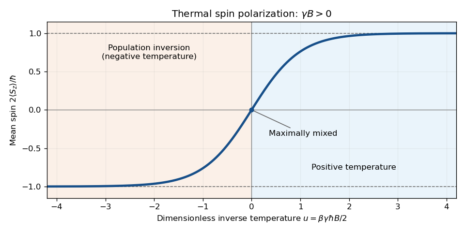
For , the quantum Gibbs state is diagonal in the basis. Its two probabilities are proportional to . ThusAt small inverse temperature, . As a function of , the normalized spin component is the smooth odd curve : it crosses zero at and saturates at . As a function of its direction is reversed if . For , positive temperature favors , while negative temperature gives the inverted population.

Past exam of the theoretical physics II course of the University of Cambridge 2017 2 d Solution 2026-10-18
Specify the magnetic coupling before fixing its sign: let the magnetic moment be , where is a signed gyromagnetic ratio. The Zeeman effect gives . For spin one-half, , so with and ,This is the quantum Gibbs state. Its eigenvalues are , so its purity is . For nonzero level splitting it approaches a pure state as : positive inverse temperature selects the lower energy, while negative inverse temperature selects the upper one. It is a maximally mixed state at , including infinite temperature or zero magnetic splitting. At zero field the Gibbs state remains ; lowering temperature alone does not select a unique pure state from that degeneracy.
Negative temperature is meaningful for an internally equilibrated spin sector with a bounded energy spectrum and population inversion. It must be sufficiently isolated from unbounded motional degrees of freedom: the oscillator's unbounded spectrum, for instance, makes its partition sum diverge at negative inverse temperature. The two-level spin partition sum itself stays finite for either sign.
Past exam of the theoretical physics II course of the University of Cambridge 2017 2 c Solution 2026-10-18
The quantum state is continuous through a sudden finite-force quantum quench, so it is still at . DefineThe new Hamiltonian operator is . The old Fock vacuum obeys , so the coherent state after shifting an oscillator equilibrium rotates with amplitude relative to the new equilibrium. In the original oscillator basis, the full state isOne way to obtain the phase is to writeand apply the displacement operator composition rule. The coherent-state oscillator expectation values giveThe position uncertainty stays . These mean values obey the forced classical equation, while the nonzero variance retains the quantum width.
Past exam of the theoretical physics II course of the University of Cambridge 2017 2 b Solution 2026-10-18
A normalized oscillator coherent state is an eigenstate of the annihilation operator, . Expanding it in Fock states givesSince , , and , the variance is . Henceindependently of the complex amplitude .
For and , the commutator is the scalar . The Baker--Campbell--Hausdorff formula therefore terminates and gives the displacement operatorBecause , applying it to the Fock vacuum yields exactly the Fock state expansion above:For a general complex , its complex conjugate is required in the annihilation term. The expression with printed in the paper is valid when is real.
Past exam of the theoretical physics II course of the University of Cambridge 2017 2 a Solution 2026-10-18
Complete the square in the potential energy. With ,The quantum harmonic oscillator is translated without changing its level spacing. If is its normalized unforced energy eigenstate, thenEquivalently, . The ground state position is centered at , and its position uncertainty remains .
Past exam of the theoretical physics II course of the University of Cambridge 2017 1 e Solution 2026-10-18
For distinct positive integers , use normalized box modes and . Their contact interaction overlaps obeyUnlike traveling ring modes, these standing modes also allow pair conversion. For the first two box modes, or any distinct pair without a third-harmonic resonance, the contact interaction between two box modes isThe last two terms change an individual mode occupation number by two while conserving total particle number. Thus the Hamiltonian operator is not diagonal in the Fock state basis, and minimizing diagonal entries alone does not find its ground state. For example, at with no dispersion, has the lowest energy , below either unmixed endpoint's .
The wording permits modes beyond the first two. For completeness, the identity givesWhen , add ; when , add . These extra terms change an individual occupation number by one and require diagonalizing the corresponding fixed- matrix as well.
Past exam of the theoretical physics II course of the University of Cambridge 2017 1 d Solution 2026-10-18
Add the one-particle energy term . It is diagonal in the same Fock state basis as the contact interaction between two ring modes. For , the ordered basis givesFor , the middle eigenvalue exceeds the mean of the two endpoint eigenvalues by , so it cannot be the smallest. The ground state is therefore if , and if , withIf , every normalized linear combination of the two endpoint Fock states is a ground state. The same endpoint argument works for general fixed , since the interaction contribution is a concave quadratic function of the mode occupation number.
Past exam of the theoretical physics II course of the University of Cambridge 2017 1 c Solution 2026-10-18
At fixed particle number , write and . The contact interaction between two ring modes has energy eigenvaluesFor , the nonnegative product is minimized at the endpoints. ConsequentlyFor this is a two-dimensional degenerate ground state subspace. instead has the unique Fock vacuum. In this projected model, putting all particles into one traveling mode avoids the extra exchange contribution paid when both distinct modes are occupied.
For the alternative coefficients, put and . Then is again minimized at , with . Evenness of is unnecessary for this result; the balanced Fock state maximizes this attractive-interaction energy instead of minimizing it.
Past exam of the theoretical physics II course of the University of Cambridge 2017 1 b Solution 2026-10-18
Normalize the ring modes as , with distinct and integers . Inserting into the contact interaction givesOrthogonality makes when , and zero otherwise: this is momentum conservation in the projected Hamiltonian operator. There is one all-mode-1 term, one all-mode-2 term, and four mixed terms with one particle in each mode. A pair conversion between distinct ring modes would require and therefore vanishes.
Using and yields the contact interaction between two ring modes,The factor four comes from two independent choices of ordering for the creation operators and annihilation operators. This is the two-mode projected model; a full ring contact interaction can also scatter particles into other modes while conserving total momentum.
Past exam of the theoretical physics II course of the University of Cambridge 2017 1 a Solution 2026-10-18
In second quantization, expand the annihilating quantized field in a complete orthonormal basis of one-particle states, . At equal times, the canonical commutation relation for bosons and the canonical anticommutation relations for fermions are, respectively,andHere is a Dirac delta distribution. Multiplying by the basis wave functions and integrating gives for bosons, or for fermions; the two-annihilator and two-creator brackets vanish in the corresponding convention.
The mode number operator and total particle number operator areThe bosonic occupation numbers are . For fermions, and the canonical anticommutation relations imply , so the fermionic occupation numbers are only and , as required by the Pauli exclusion principle.
Keeping only two modes later is a projection: the projected field bracket is , rather than the full Dirac delta distribution.
Past exam of the theoretical physics I course of the University of Cambridge 2022 4 e Solution 2026-10-18
Above the threshold, , the square root in part (d) is real. Both fields oscillate, but the first has envelope and the second . Thus the first is damped and the second amplified.
Below the threshold, set . The temporal factors areThey are nonoscillatory. For nonzero , , so both first-field branches decay and both second-field branches grow. At , one branch is constant; the other is for or for .
At equality, the repeated temporal root gives for the first field and for the second. The full two-field system is generically unstable on both sides because of the amplified sector. This is compatible with its autonomous Lagrangian: the total conserved energy is an indefinite quadratic form, rather than a positive energy forcing every component to remain bounded.
Past exam of the theoretical physics I course of the University of Cambridge 2022 4 d Solution 2026-10-18
The velocity coupling changes the momenta and the undifferentiated field terms. Variation with respect to gives the equation for :so the two Euler-Lagrange field equations areThey describe damped and antidamped fields from an antisymmetric velocity coupling. With the convention , their characteristic equations areThus the dispersion relations and modes areFor each spatial Fourier mode, the general solution is the linear combination of its two temporal branches; spatial superposition gives the general field. Take real parts or suitable complex conjugate pairs to obtain the required real fields. At the repeated-root threshold, the independent second temporal solution contains an extra factor , as detailed next.
Past exam of the theoretical physics I course of the University of Cambridge 2022 4 c Solution 2026-10-18
Use coordinates , and first compute the mixed canonical stress-energy tensor supplied by spacetime translations:Define the energy density and . Direct substitution givesThe two wave equations implyFor example, differentiating and replacing each by gives exactly by the product rule. These are respectively the two component equations , establishing stress-energy conservation explicitly.
If the given metric is used to raise the second index in these unrescaled coordinates, the result is , still conserved. To display the symmetric relativistic form with light speed , choose , instead. With , the corresponding tensor isThis states the coordinate convention explicitly rather than setting in some components but not others.
Past exam of the theoretical physics I course of the University of Cambridge 2022 4 b Solution 2026-10-18
The infinitesimal connected internal symmetry of a classical field theory is , . For this exact invariance of the Lagrangian density, the Noether current is . In coordinates it isVarying the two fields gives the two wave equations and . Direct differentiation cancels the first-derivative cross terms:The Noether charge is constant when the spatial boundary flux vanishes. The disconnected transformations from part (a) do not have independent infinitesimal generators of this type.
Past exam of the theoretical physics I course of the University of Cambridge 2022 4 a Solution 2026-10-18
Apply the linear transformation of the scalar fields to either time- or space-derivative product. Its coefficients become multiplying the square of the first derivative, multiplying the square of the second, and multiplying their cross product. Invariance for arbitrary fields therefore requiresThe complete real solution isThere are four connected components, distinguished by the diagonal/antidiagonal choice and the sign of . Only the positive diagonal family is in the identity component; write to obtain , . This is the reciprocal rescaling symmetry of two cross-coupled scalar fields. The antidiagonal transformations exchange the fields as well as rescale them.
Past exam of the theoretical physics I course of the University of Cambridge 2022 3 g Solution 2026-10-18
For a homogeneous saddle-point approximation define . With the cubic source coupling, minimizing the Landau free energy givesIts curvature is positive, so there is a unique local minimum and global minimum. The solution near hasbecause substituting this leading term makes the cubic self-interaction of order . Therefore the cubic source coupling and third-order susceptibility giveThus the first nonzero response diverges like from above. The factor is essential: the coefficient of is not itself the third derivative. This is susceptibility to the specified cubic source variable, rather than the usual third-order response to a linearly coupled field.
Past exam of the theoretical physics I course of the University of Cambridge 2022 3 f Solution 2026-10-18
The coarse-grained order parameter is a real scalar field because the microscopic spin has one component. At , spin inversion symmetry takes , so an analytic local Landau free energy contains only even powers. Near a continuous phase transition, the quadratic coefficient changes sign linearly, represented by with . A positive quartic coefficient stabilizes the density when the quadratic term becomes negative, giving the two minima below .
The ferromagnetic interaction favours neighbouring spins pointing alike, so spatial variation costs energy; its leading long-wavelength form is the positive gradient term . The source term favours alignment with the applied magnetic field and explicitly breaks spin inversion symmetry at fixed nonzero . Finally is the spin-independent background free-energy density.
The quartic sign can also be checked from part (b): its expansion containswhose quartic coefficient is positive. This is consistent with the proposed Landau-Ginzburg theory, not a tricritical truncation requiring a stabilizing sixth-order term. The microscopic square lattice is two-dimensional; the written gradient describes a profile depending on one coordinate. For general profiles, replace it by .
Past exam of the theoretical physics I course of the University of Cambridge 2022 3 e Solution 2026-10-18
The small-argument Taylor series of the single-site response isLet . For a small nonzero order parameter at zero field, the self-consistency equation becomesSince and , where , this givesConsequentlyThe positive branch is the expression printed in the question, while its negative partner is required by spin inversion symmetry. The square-root behavior gives the mean-field critical exponent for the spontaneous magnetization.
Past exam of the theoretical physics I course of the University of Cambridge 2022 3 d Solution 2026-10-18
At zero field, write the right-hand side of the self-consistency equation as , with . The origin is always a solution, and the slope there isThe critical crossing occurs when this equals one, givingThis is a continuous phase transition in the mean-field approximation. For ,so the positive branch is a strictly concave function, while is odd and bounded by one. For , the slope at zero is at most one and strict concavity puts below for every , leaving only the unmagnetized solution. For , it initially lies above but has ; hence there is one positive intersection and, by spin inversion symmetry, one negative intersection.
The curvature of the Helmholtz free energy in the mean-field approximation is per site. It is negative at below and positive at the nonzero intersections, identifying the ordered minima and the unstable zero solution.
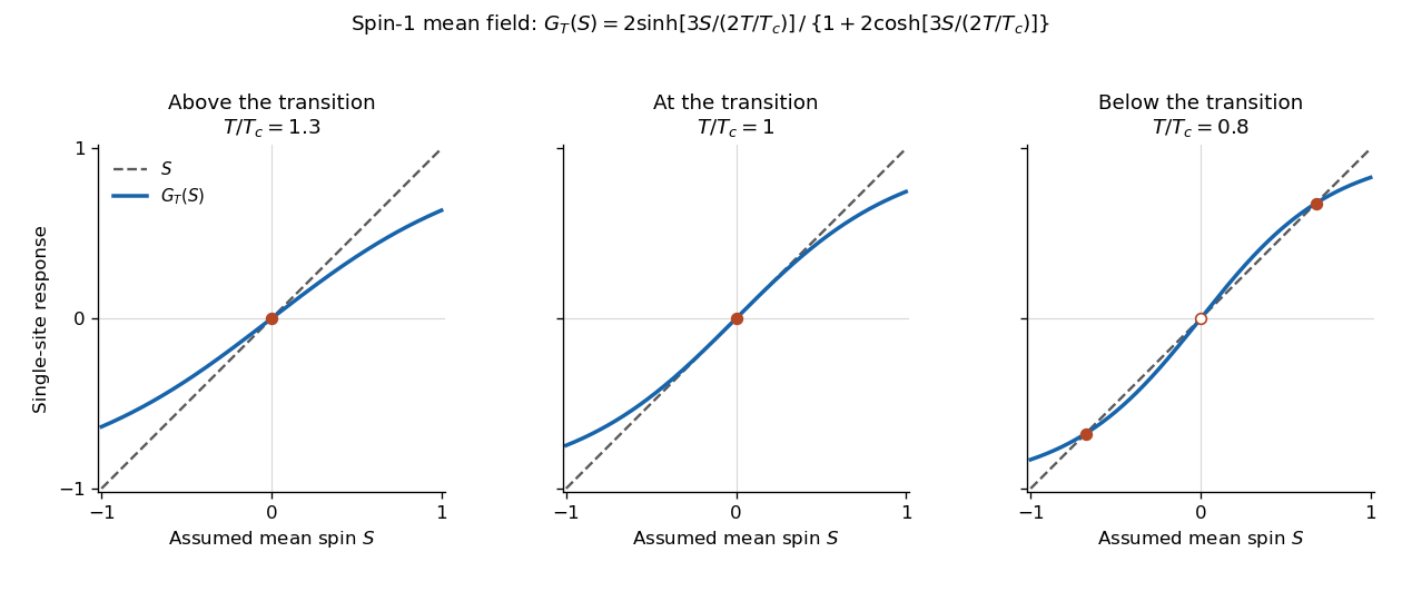
The self-consistency equation develops two nonzero order parameter branches below the mean-field critical temperature
. Details. 
The critical temperature and branches here belong to the mean-field approximation. In the exact finite system, spin inversion symmetry forces zero average magnetization at zero field; selecting a broken-symmetry phase requires the thermodynamic limit with a vanishing field of specified sign.
Past exam of the theoretical physics I course of the University of Cambridge 2022 3 c Solution 2026-10-18
The self-consistency equation requires that the mean spin computed using the single-site Boltzmann distribution equals the spin used to form the effective field. With ,ThusEquivalently, differentiating part (b) gives , so stationarity of the Helmholtz free energy in the mean-field approximation is exactly this condition. Among multiple stationary points one must select the stable minimum.
There are unlisted articles, also show them or only show them.