
Near order , the first angular zero from a principal maximum is . Two wavelengths have peak separation . Equating them applies the Rayleigh criterion and gives the resolving power of a diffraction grating,Here the required resolving power is , so in second order . The illuminated width is thereforeWhether one counts the full illuminated window or the first-to-last slit-centre distance changes the width by one pitch and is immaterial at this precision. The result assumes negligible aberrations and adequate slit illumination and coherence.
The pitch corresponding to is . The normal-incidence diffraction grating equation givesThis locates the array-factor maximum; the single-slit envelope must also be nonzero for an observable peak.
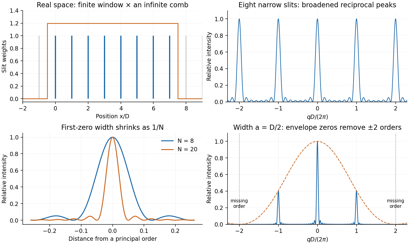
Use Fourier transform convention . The convolution theorem givesA finite array of very narrow slits at , , has transmission proportional to . It can be constructed by multiplying an infinite Dirac comb by a finite window. The infinite comb transforms to a reciprocal comb; the finite window convolves each reciprocal peak with a narrow sinc-shaped amplitude. Thus increasing the illuminated length narrows each Fraunhofer diffraction peak.
The exact finite sum makes the argument quantitative:Its normalized intensity is . Principal maxima occur at ; their first zeros are displaced by . Replacing the ideal narrow slit by a finite slit function convolves the array in real space, multiplying this field by the single-slit Fourier transform. Field amplitudes are transformed and combined before their squared modulus is taken.
Taking as the distance travelled in the medium, the narrowband group delay isIf denotes a slab thickness measured normal to the interface instead, the central ray travels , giving about . The coordinate-mixed velocity above would give for a path; it should not replace the consistent calculation silently.
The pulse envelope travels at the local group velocity, while individual carrier crests move at the phase velocity. In general, variation of group velocity across the pulse spectrum produces different delays, temporal broadening and chirp. Absorption can reshape the spectrum and envelope as well. The refraction data also show wavelength-dependent angles, so a finite-width incident beam acquires spatial separation of its spectral components. The supplied first derivative determines the central delay but does not specify a pulse duration, absorption spectrum or reliable second derivative of the dispersion relation; it therefore does not determine a numerical broadening, or its sign. If propagation phase is effectively linear across a sufficiently narrow spectrum, the leading approximation is a delayed pulse with unchanged shape.
The wavelengths specified for incidence from vacuum are . With fixed incident angle , Snell's law gives and . At the central wavelength,Use a central difference, converting the angle change to radians:The group index from refracted-angle dispersion isDirectly inserting the incident vacuum wavelengths into would instead give . That is a plausible intended rough answer, but it mixes wavelength coordinates; the boxed result consistently uses the incident data. The two agree only to first order in a sufficiently small dimensionless dispersion correction.
For the wavelength in the medium, , differentiate :The distinction in group velocity in material and vacuum wavelength coordinates is essential for the numerical data. For incident vacuum wavelength , differentiation of instead givesThus the printed derivative identity is valid, but its wavelength coordinate cannot be carried unchanged into data specified before refraction.
Superpose two nearby harmonic waves. The identityseparates a rapid carrier from a slow beat envelope. A constant point of the envelope moves at , which tends toas the components approach one another. Equivalently, expand a narrow wave packet spectrum around : . Factoring the carrier out of its Fourier transform representation leaves an envelope depending on . This interpretation requires a narrow spectrum and little attenuation or distortion; higher derivatives of the dispersion relation can change the envelope shape. The carrier phase velocity is and need not equal .
To settle quickly after loading, critical damping is preferable to the supplied weak damper:Using the strict-bound mass instead changes this by less than . This eliminates free ringing while avoiding the slow tail of severe overdamping. In the stipulated external-force model, greater damping also reduces the steady forced amplitude; there is no finite optimum based solely on that amplitude. A critical or near-critical value is a practical compromise for rapid settling. If the disturbance were specified as floor displacement transmitted through the legs, damping would introduce an additional transmission tradeoff, but that is a different forcing model.
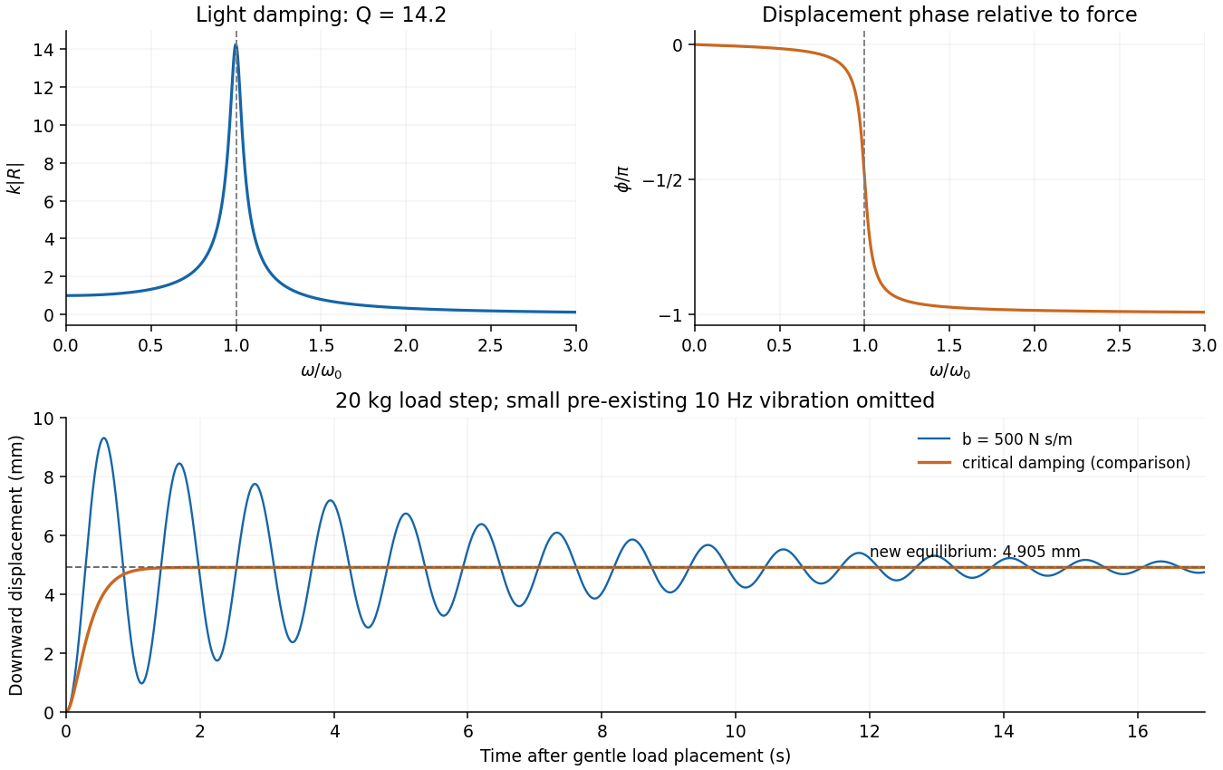
Measure downward displacement relative to the former mean equilibrium. The added changes the equilibrium byAssume the load is deposited without a significant impact impulse and then moves with the table. The moving mass becomes . Ignoring the tiny pre-existing vibration in the sketch, the added-load step response of a supported table isFor the estimated mass, , the envelope time is , and the period is about . The table overshoots and rings about the new equilibrium, with the displacement starting continuously at zero and with zero initial slope. A real impact adds an initial-velocity transient; the problem gives no impact history. The residual driven vibration, of order a micrometre, can be superposed.


The four supporting springs act in parallel, so their total spring constant is . The driving angular frequency is . The force-driven vibration isolation estimate givesAt this mass, , and , so the assumptions are consistent. The exact forced amplitude isIt is indeed close to , but it is slightly above the strict requested bound. Setting the exact expression to gives the high-mass thresholdChoose a mass strictly greater than this threshold for a strict inequality; is a suitable rounded choice. Simply rounding the high-frequency estimate down would not guarantee the bound.
To find the displacement peak, minimize the squared denominator:The nonzero minimum givesFor stronger damping there is no positive-frequency displacement maximum. When and ,The inertia then dominates the restoring and damping forces.
Use the convention for the harmonic force and displacement complex amplitudes. Substitution in the forced harmonic oscillator equation givesIts magnitude and phase relative to the force areAt zero frequency, and . At , ; at high frequency the phase approaches . For light viscous damping, the quality factor is large and there is a tall narrow displacement peak close to .
A Gaussian distribution with mean and standard deviation has probability densityIts symmetry, finite variance and simple behavior under linear combinations make it useful for repeated measurements. Roughly , and of observations lie within one, two and three true standard deviations of the mean. These are coverage probabilities for a specified distribution, not guarantees that every experimental error is normal.
Why it appears. The central limit theorem explains why many sums of small independent finite-variance contributions approach a Gaussian law after centering and scaling, provided no single contribution dominates. Detector noise, small mechanical disturbances and multiple electronic fluctuations can combine approximately this way. The theorem does not remove a common calibration bias, and it does not justify assuming normal tails for rare large disturbances or arbitrarily correlated errors. A large-mean Poisson distribution also approaches a Gaussian with variance equal to its mean, making normal approximations useful for high-count photon or particle data; low counts require the discrete model.
A classical particle at thermal equilibrium in a one-dimensional harmonic potential has a Gaussian position distribution directly from the Boltzmann distribution:Thus a Gaussian law can arise from the energy dependence of equilibrium probability, rather than only from an informal appeal to many independent errors.
Precision of repeated measurements. For independent observations with the same mean and variance, the sample mean has variance . For Gaussian observations this mean is exactly Gaussian:Consequently quadrupling the number of independent readings halves the random standard error. When the true variance is unknown, a small-sample confidence interval for a normal mean uses a Student t-distribution with statistical degrees of freedom; replacing that by a normal quantile can overstate precision. Shared systematic errors and correlations do not decrease by the same averaging rule.
Combining results and fitting models. Independent Gaussian estimates of one quantity, with known variances , combine through the inverse-variance weighted meanFor a model with independent zero-mean Gaussian noise, maximizing the likelihood is equivalent to minimizing the weighted least-squares statisticFor a correct linear model with known independent Gaussian errors and fitted parameters of full rank, the minimized statistic has a chi-squared distribution with degrees of freedom. Nonlinear fits only inherit that familiar approximation under additional regularity and adequate-data assumptions. Known correlated Gaussian errors require the full inverse covariance matrix in the quadratic form.
These properties support confidence intervals, consistency checks, calibration and error propagation. They also give practical diagnostics: inspect residuals for trends, changing spread, correlations or outliers before trusting a Gaussian fit. Gaussian models connect physical fluctuations to quantitative uncertainty, but their assumptions must be checked rather than inferred from the shape of a convenient bell curve.
In this digital-sampling context, Nyquist's theorem means the Nyquist–Shannon sampling theorem. A continuous signal with no Fourier content outside can be reconstructed from uniformly spaced samples taken sufficiently fast. The familiar practical condition isHere is the Nyquist frequency, while is the Nyquist rate required by that signal bandwidth. A finite-energy bandlimited formulation allows equality; a rule intended to include arbitrary pure sinusoids at the boundary must be strict, because vanishes at every sampling time .
The mechanism is visible in the Fourier transform. Sampling by a time comb creates shifted copies of the original spectrum, separated by :If those copies do not overlap, an ideal reconstruction filter selects one copy and recovers the original waveform. Equivalently, ideal interpolation uses the normalized sinc function:Each interpolation function is one at its own sample and zero at all other sample times. Exact reconstruction presumes the bandwidth condition, an ideal sampling clock and the full sample sequence.
If the spectrum extends beyond half the sampling rate, different continuous frequencies become indistinguishable: this is aliasing. A sinusoid at frequency is indistinguishable on the sampling grid from frequencies differing by integer multiples of , with the usual sign reflection for real signals. For example, sampled at aliases to ; a later digital filter cannot tell which signal generated those samples.
Use an analogue anti-aliasing filter before the analogue-to-digital converter and choose a sampling rate leaving room for its finite transition band. Faster sampling can relax that analogue filtering problem, but simply increasing the number of samples in a fixed-duration record does not improve the independent Fourier-bin spacing beyond approximately . A long recording is needed for low-frequency resolution, while a small sampling interval is needed for high-frequency coverage. Finite records also introduce windowing and spectral leakage.
Digitization adds amplitude quantization as well as time sampling. An ideal -bit converter spanning voltage range has step . When quantization error may be modeled as independent and uniform across one step, its rms size is ; small coherent signals need not obey that white-noise approximation. Sampling rate controls temporal ambiguity, recording duration controls frequency resolution, and converter resolution controls amplitude discretization.
Electrical noise reduction starts by identifying what is unwanted in the measured signal and where it enters. Increasing gain amplifies both signal and input noise; it does not by itself improve the input signal-to-noise ratio. Separate intrinsic component fluctuations, amplifier noise and external pickup before choosing a remedy.
Physical sources. A resistor at temperature has classical one-sided open-circuit thermal electrical noise density per hertz. In a flat measurement bandwidth , its rms voltage is . Lowering an appropriate resistance, reducing temperature or narrowing the useful bandwidth can reduce this noise, with loading and signal-gain tradeoffs considered. These are power spectral densities; an amplitude spectral density is their square root.
Discrete independent charge transfers give shot noise, with one-sided current density in the simple Poisson process model. Reducing leakage or unwanted bias current can help, but reducing a photocurrent may also reduce the desired signal. Charge correlations can change the simple shot-noise law. At low frequency, flicker noise and drift often dominate and are not described by a white spectrum.
Amplifier and impedance choice. An operational amplifier has equivalent input voltage and current noise. In a simplified uncorrelated model, a resistive source contributes the input-referred voltage densityHere are the voltage and current amplitude spectral densities and is the source electrical impedance; feedback components add further terms in a full circuit. Low current noise matters particularly for a high-impedance source, while voltage noise can dominate for a low-impedance source. Minimize needless source impedance, leakage and long sensitive connections without sacrificing the required transduction gain or bandwidth. Bias-current offsets and thermal drift also require calibration; they are not removed simply by quoting a random-noise density.
Pickup and bandwidth. Shield sensitive circuits against electric-field coupling, minimize loop area to reduce changing magnetic-flux pickup, and use twisted signal/return pairs or suitable coaxial connections. Differential readout rejects common-mode interference when impedances and amplifier responses are adequately matched. Plan the signal returns to avoid unwanted circulating ground currents, and decouple supply rails locally so supply fluctuations do not enter the signal path. Mechanical vibration, cable motion and temperature changes may be converted into electrical noise as well.
A low-pass filter removes out-of-band noise before digitization; an anti-aliasing filter is needed because digital filtering cannot undo already aliased content. Avoid a narrower passband than the physical signal requires. For a known periodic signal, modulation and a lock-in amplifier select a narrow frequency interval, often moving the measurement above a strong flicker noise region. A notch can reject a narrow interference line if that does not remove essential signal information.
Independent noise contributions add in variance, not directly in rms amplitude. Averaging independent equal-variance readings reduces the standard error by , but slow correlated drift and systematic errors need separate controls. Good noise reduction preserves the information-bearing signal while reducing unwanted coupling, intrinsic fluctuations or the admitted noise bandwidth.
A Hermitian operator satisfies the adjoint symmetry conditionfor vectors in its specified domain. For a finite matrix this means . For an unbounded differential operator, boundary conditions and domains matter: symmetry on a chosen domain is not alone sufficient for self-adjointness. Physical observables require the corresponding self-adjoint operator and its spectral measure. This distinction prevents purely formal integration by parts from being mistaken for a complete operator definition.
Real eigenvalues. If with nonzero norm, Hermiticity impliesso . Thus eigenvalues representing measurement outcomes are real.
Orthogonality. For eigenvectors ,Hence , and distinct eigenvalues have orthogonal eigenvectors. Within a degenerate eigenspace, Gram-Schmidt orthogonalization can choose an orthonormal basis. In finite dimensions the spectral theorem gives a complete orthonormal eigenbasis andwhere projects onto each eigenspace. In infinite dimensions a continuous spectrum may require a spectral integral rather than a normalizable eigenvector for every possible outcome; a position operator on the full line is a familiar example.
Measurements and probabilities. In the discrete case the Born rule assigns probability to the outcome . For a nondegenerate eigenbasis, gives probabilities , withThe variance vanishes precisely when the state lies in an eigenspace with a single sharp outcome. A repeatable ideal projective measurement prepares the corresponding eigenspace; superpositions of different eigenvalues do not have a preassigned sharp value of that observable in this description.
Compatibility and dynamics. Commuting Hermitian matrices admit simultaneous diagonalization, permitting a common set of sharp labels. For example commute, whereas do not. In the differential-operator setting the corresponding spectral compatibility requires appropriate domain conditions. Noncommuting observables obey the Robertson uncertainty principleThe canonical commutation relation then gives .
The Hamiltonian operator represents energy. A self-adjoint generates unitary time evolution, , preserving norm and total probability; its eigenvalues determine stationary-state phases and transition energies. Hermiticity supplies real outcomes and orthogonal eigenspaces, while self-adjointness and the spectral theorem make these measurement and evolution rules mathematically complete.
Ehrenfest theorem relates the dynamics of quantum expectation values to operator commutators. For a normalized state obeying and a possibly time-dependent observable , differentiate . Using the adjoint Schrödinger equation for the bra givesThusThe identity assumes a common domain on which the required products and derivatives are defined.
For , the canonical commutation relation gives and . ThereforeThese resemble Hamilton's equations and Newton's second law, but generally . If the state is localized about , a local expansion givesThe classical trajectory equation for the mean is accurate when the force changes little across the wave packet. For a quadratic harmonic potential, is linear and this closure is exact for every state with the relevant finite moments: . This exact classical evolution of the centroid does not eliminate its quantum position uncertainty or make every state a point particle.
The correspondence principle is broader: quantum predictions recover classical ones in an appropriate limit, such as large action compared with and observations that cannot resolve individual quantum levels. It is not the assertion that every large quantum number automatically makes every possible state classical. Delocalized superpositions and interference can remain significant unless the physical preparation and measurement justify a classical description.
A spectral example is useful. For a quantum harmonic oscillator, neighboring levels differ by , giving transition frequency , equal to its classical oscillation frequency. A coherent state makes the connection more concrete: its mean position and momentum oscillate classically while the finite-width Gaussian profile retains its quantum uncertainty. For hydrogenic Bohr levels , transitions between nearby large have , which equals the classical circular orbital angular frequency in that model. Ehrenfest's theorem supplies an exact expectation-value bridge; a classical trajectory follows only when the force can also be evaluated at the mean position.
The Bohr model combines classical circular motion in the Coulomb potential with explicitly quantum postulates. A one-electron atom of nuclear charge has electron–nucleus reduced mass . With , the relative circular orbit obeysBohr postulates permitted nonradiating stationary orbits with , for . These assumptions giveFor hydrogen with the nucleus taken infinitely heavy, the radius is the Bohr radius, . The finite reduced mass gives the small nuclear-motion correction, and increasing contracts the one-electron orbit.
The circular-motion equation gives while the potential energy is , so the total energy is . Substituting the quantized radius yieldsFor the heavy-nucleus hydrogen approximation, . The ionization threshold is zero energy, so removing the ground-state electron requires about .
The model further postulates that radiation is emitted or absorbed only in transitions between stationary orbits, with photon energy . Emission from givesThus it reproduces the principal hydrogen spectral series, their limiting wavelengths, and the gross hydrogenic energy levels. For example, in hydrogen has and , a visible line. Absorption reverses the transition when the photon matches the energy gap.
The achievement is that quantized energies explain discrete spectra, but the model's stationary orbits are postulates rather than consequences of classical electrodynamics: an accelerating classical charge would radiate. It does not provide a general calculation of line intensities or transition selection rules and fails as a quantitative theory of many-electron atoms. Spin, fine structure and the full Zeeman effect require further physics. Modern quantum mechanics replaces definite electron orbits by wavefunctions and quantum probabilities. In particular, the true hydrogen ground state has , so its orbital angular momentum vanishes; the model's rule should not be identified with the modern orbital eigenvalue rule . Bohr's energy quantization remains a successful hydrogenic approximation, while its literal orbital picture does not.
Using the observed counts,ThusTogether with the direct ground state branch, these sum to unity. No measurement uncertainties were supplied for these ratios, so the extra digits only document the arithmetic.
Let be the common normalization converting the quoted to photon numbers per parent decay. Apply nuclear level population balance to scheme A, starting with the top level:For example, the transition contributes to the population of level 2; it must be subtracted from the total leaving level 2 to obtain its direct beta feeding. Similarly, a photon in the strong line need not imply a direct beta transition to level 1.
The three equations giveAdding them cancels the internal cascade counts:This also has a simple physical meaning: each decay that initially feeds an excited daughter eventually contributes exactly one of the three transitions into the ground state. The number of all emitted photons is not the correct normalization, because a single cascade can emit several.
Consequently the required formulae are
There are unlisted articles, also show them or only show them.