
Add the particular solution to the complementary function. The real general solution isThe five constants remain arbitrary until initial data are specified.
A quadratic polynomial is sufficient: set . Its fifth derivative vanishes, so . Matching the forcing gives , hence a particular integral is
In the homogeneous equation, substitute the exponential function . The characteristic equation isIts distinct roots are . Combining the complex-conjugate pair into real sine and cosine gives the complementary functionFive linearly independent terms supply the required five homogeneous degrees of freedom.
After integrations, the general solution is an arbitrary polynomial of degree at most :Conversely, every such polynomial has zero th derivative. The free coefficients span the full solution space on a connected interval.
Integrating once gives a constant first derivative, and integrating again givesThere are two independent constants, as expected for a second-order ordinary differential equation.
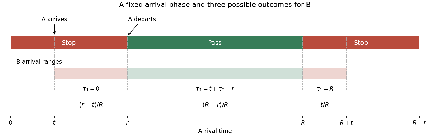
The remaining arrivals occur in the next stop phase: , or . B waits until , while A departed at , giving . This interval has length , henceEndpoint assignments do not affect probabilities. The three outcomes are exhaustive and satisfyThese are conditional probabilities for the stated fixed ; there is no additional averaging over A's arrival phase in the question.
Condition throughout on the given arrival time of A, with . A departs at time . B also departs at exactly when it arrives before that release, so , or . Since is uniform on an interval of length ,The original timeline below shows the three disjoint ranges of . The same idealized simultaneous-release convention as in part (a) is used.
The second moment isSubtracting the squared expected value gives the variance and standard deviation:The variance is nonnegative because . Both and have units of time. At the result reduces to , the standard deviation of a uniform distribution over one full cycle.
The probability of a positive delay is the integral of its density:Adding the separate no-delay event givesThis is the normalization of a probability distribution with both discrete and continuous parts.
The graph of the positive-delay probability density function is a horizontal segment at height from to , followed by zero from to . Values at individual endpoints do not affect probabilities. The separate atom at zero is not a finite-height part of this density graph.
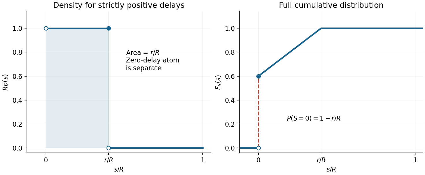


The companion cumulative distribution function in the figure is for , for , and for . Its jump at zero displays the discrete part without confusing density height with probability mass.
For a stop-phase arrival at time , the delay is . An interval of delays of width therefore corresponds to an interval of arrival phases of the same width, because . Its unconditional probability is . Hence the positive-delay part has densityThis ordinary density integrates to , not to one: the remaining probability mass is at . Thus has a uniform distribution with an atom at zero, with mixing weight . Conditional on a positive delay, the density would instead be on .
The arrival phase has a uniform distribution over a cycle of length . The no-delay phases occupy length , soIndividual phase endpoints have probability zero. The model neglects clearance time and releases waiting vehicles together when the stop interval ends; the degenerate case is interpreted as release at successive cycle boundaries.
Since , substitute the proposed inverse series into the forward one. Comparing coefficients of givesSolving successively yields the cubic series reversion coefficientsThe conditions and ensure that both local series are centred at zero and that the inverse has a linear leading term.
Assume the needed derivatives exist continuously and on a neighborhood, so the inverse function theorem provides a local inverse. Put , , and . The chain rule gives , soDifferentiate once more:Thus the first three derivatives of an inverse function areAll forward derivatives on the right are evaluated at the corresponding value .
Use . The Maclaurin series givesAll three nonzero terms are needed; stopping at fourth order would supply only two.
The derivative of the inverse tangent is . Expand it as a geometric series and integrate term by term near zero, using :
Expand the natural logarithm and reciprocal separately:Multiplication gives the first three nonzero terms of the Maclaurin series:The local expansions converge for .
Summing the diagonal entries givesThe eigenvalues of the inverse are the reciprocals of those of , whose sum is also . This is precisely what the trace identity predicts.
There are unlisted articles, also show them or only show them.