
A rational lower bound for the natural logarithm proves positivity for every , including . DefineThen , while direct differentiation givesThus for . Setting in the expression from part (b) givesTherefore , and is a strictly increasing sequence.
For , the Taylor series of the natural logarithm converges absolutely at :Multiply this power series by and subtract . The constant term cancels the subtracted , and the coefficient of is . For , the coefficient of isHenceIn particular , in Big O notation.
Cancellation of the factorials in the consecutive ratio givesSet . The derivative of the natural logarithm at gives . ThereforeThus the necessary condition from the term test for divergence is satisfied. On its own it does not prove that converges.
All are positive, and . The logarithm turns consecutive ratios into differences, producing the finite telescoping sumThus, already for every finite ,If the partial sums converge to , the continuity of the exponential function givesThe shift from to preserves the limit of a sequence. Convergence of the partial sums is established in part (f), so no convergence assumption is left unsupported.
At , all odd-indexed cosine terms vanish, while . Thus the Fourier series from part (c) givesDivide by and rearrange. The hyperbolic sine identity yieldsThe evaluation is legitimate by the convergence established in part (c).
The function is even, so each product with a sine is an odd function and all the Fourier coefficients vanish. Its constant coefficient isFor , part (a) gives the remaining Fourier coefficients:Consequently the Fourier cosine series isThe periodic extension is continuous, including at , and piecewise continuously differentiable. Thus the Fourier series equals everywhere. Its coefficients are also bounded in magnitude by a constant times , which gives absolute convergence.
A Fourier series represents a periodic function as a constant plus sine and cosine waves whose frequencies are integer multiples of its fundamental frequency. For period , use the conventionwhere the Fourier coefficients areThe coefficient formulas follow by multiplying by a basis sine or cosine and using their orthogonality over a full period. A Fourier series need not equal an arbitrary function at every point. The pointwise convergence of a piecewise smooth Fourier series theorem says that for a piecewise continuously differentiable function, the Fourier series converges at each point to the average of the two one-sided limits, and hence to wherever is continuous.
From part (f), . To obtain , choose the Householder transformation that reverses only the third coordinate:Indeed , so , and direct matrix multiplication gives . The alternative vector produces the same matrix. Geometrically reflects in the plane , completing the reversal of all three coordinates.
The second matrix acts byApplying from part (e) then givesThe Householder transformation reflects in the plane . Its normal vector is perpendicular to , so the two reflecting planes meet at a right angle along the axis. Their composition is a rotation through about the axis, as is also immediate from the displayed rotation matrix.
The matrix issoHere , so with . This is a Householder transformation: reflection in the plane . The component parallel to the normal vector changes sign, while the perpendicular component is fixed.
Using Einstein notation and the Kronecker delta,The unit vector condition is essential in the last step.
Apply matrix multiplication to obtainSince is a unit vector, the subtracted term is the orthogonal projection of along . Hence is the orthogonal projection onto a plane through the origin with normal vector . It fixes every vector perpendicular to and sends every scalar multiple of to zero. In particular .
By the definition of matrix multiplication and trace, with all indices summed from to ,The entries are scalars, so their multiplication commutes. Reordering them and renaming the summed indices givesEquivalently, in Einstein notation, . This proves the cyclic property of the trace.
The gradient isIt is perpendicular to each nonzero level set and points towards increasing . Near the two positive local maxima, the Hessian matrix is , so the gradient arrows point inward. Near the two negative local minima, the Hessian matrix is , so they point outward. These arrows are shown on the figure in part (c).
At the saddle point, . Along , the arrows point away from the centre on both sides; along , they point towards the centre on both sides. On the positive axis they point up, on the negative axis down, on the positive axis right, and on the negative axis left. This specifies the four intervening sectors of the gradient pattern.
In the translated coordinates , , the zero level set is the pair of lines and . The function is positive in the quadrants and negative in those with , and tends to zero as . Thus its nonzero contours form closed curves around the four off-centre stationary points.
For an explicit description of the contour plot, use polar coordinates , :At fixed direction within a quadrant, the magnitude increases until and then decreases towards zero. Also , with equality exactly when , and similarly for . Consequently ; each positive level below encloses a positive peak in each positive quadrant, with the analogous negative contours in the negative quadrants.
To classify the stationary points, the Hessian matrix isAt it is , with eigenvalues and , so is a saddle point. At it is . Therefore and are strict local maxima, and and are strict local minima. These are also global maxima and minima by the bound just proved.
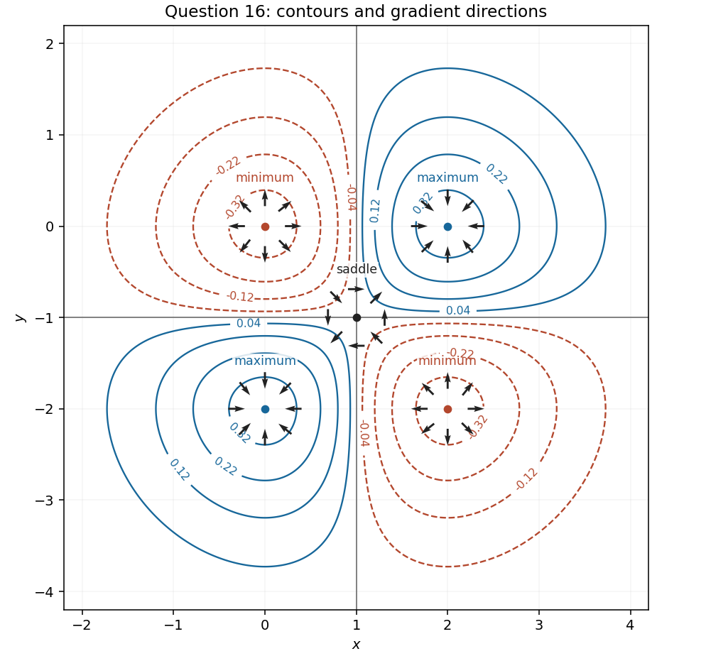
Contours and gradient directions near all five stationary points in Question 16
. Details. 
There are unlisted articles, also show them or only show them.