
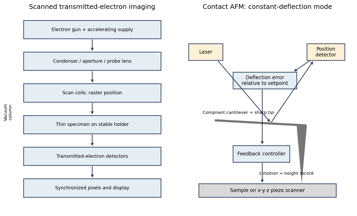
A scanning transmission electron microscope makes an image by assigning a transmitted-electron signal to each position of a scanned probe. Its essential chain is electron source, probe-forming optics, scan system, thin specimen, transmitted-electron detectors and synchronized acquisition.
An electron gun and accelerating supply provide a stable beam of the chosen kinetic energy. Condenser lens optics and an aperture control probe current and convergence; the probe-forming objective lens focuses a small spot on the specimen. Alignment, focusing and astigmatism correction keep the probe usable across the field.
Scan coils deflect the probe in a raster. A stable specimen holder positions an electron-transparent region, and a high-vacuum column limits gas scattering and contamination. A bright-field transmission electron microscopy detector collects the central transmitted beam; an annular detector can select annular dark-field electron imaging, including high-angle annular dark-field imaging. Different angular selections give different contrasts, rather than a universal map of height.
Detector electronics, scan timing and a computer assign the collected signal to the corresponding image pixel. Spectrometers are useful additions but not essential to basic image formation. The post-specimen optics can adjust detector collection geometry; they do not set scan-image magnification in the same way as the projection lenses of conventional transmission imaging.
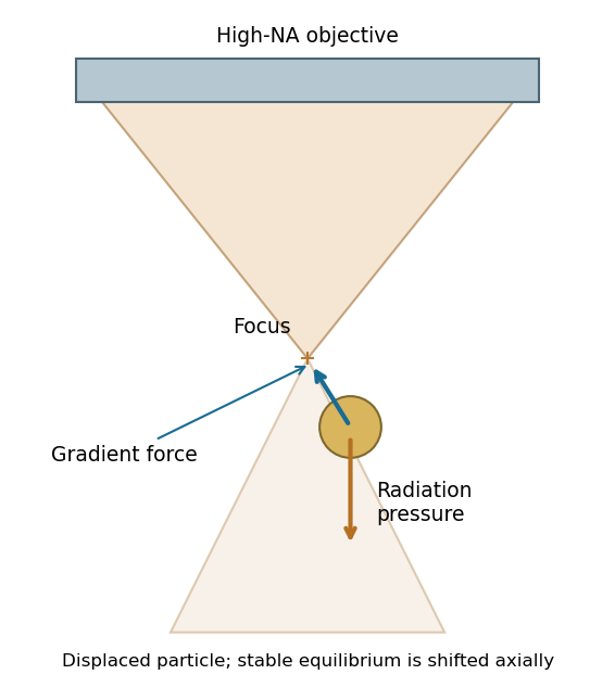
A tightly focused laser produces a strong intensity gradient. A small polarizable particle experiences a gradient force toward increasing intensity when the real polarizability has the appropriate positive sign; radiation pressure from scattering and absorption pushes predominantly along the beam. A high-numerical-aperture objective creates lateral confinement and a sufficiently strong opposing axial gradient for a three-dimensional optical trap. Equilibrium is generally shifted from the intensity maximum by radiation pressure.
For a Rayleigh sphere, in an absolute-permittivity convention, and for peak complex field amplitude. Near a stable point, ; the trap depth must exceed thermal fluctuations sufficiently to retain the particle. Viscous drag opposes motion, Brownian forcing produces fluctuations, and gravity/buoyancy are normally small at this scale.
For absorbing gold, use its complex wavelength-dependent permittivity: scattering, absorption and heating can frustrate trapping. The existence of an ideal dielectric gradient-force trap does not guarantee stable trapping of every metal nanoparticle at every wavelength or power.[ref]
Observation of a single-beam gradient force optical trap for dielectric particles by Arthur Ashkin and others. General optical trapping principle; gold-specific absorption qualification is separate
Interpreting the nominal size as diameter , fluid viscous dominance requireswith in . The liquid density is not supplied, so the conventional fluid-Reynolds crossover is not numerically fixed. As an explicitly additional illustrative assumption, gives near ; ordinary much slower nanoparticle motion is well within the viscous regime.
If instead the supplied gold density is inserted into the dimensionless ratio , that ratio reaches one at . It is not the fluid Reynolds number. Including the spherical Stokes prefactor, the particle relaxation criterion occurs at . These quantify different inertia comparisons. The wording's speed direction is reversed: viscous dominance is obtained by making speed sufficiently small. If 10 nm denotes radius, the length-based thresholds halve.
For fluid density , speed and characteristic length , inertial kinetic energy scales as while viscous work over distance scales as . Their ratio is the Reynolds number,Smaller particles at a fixed speed have smaller Re, so viscous stresses dominate fluid inertia when . Increasing speed increases Re and eventually makes inertia more important, rather than making viscous dominance stronger.
Particle inertia is a separate issue. Its particle velocity-relaxation time is ; comparing it with a travel time gives a Stokes number . This uses particle density , whereas the fluid Reynolds number uses fluid density .
For radius and gold density , . The supplied Stokes model gives and at . Therefore the standard one-second diffusive rms distances are in one coordinate and in three dimensions.
Using the source's supplied shorthand literally with instead gives . That shorthand lacks the factor two in the standard long-time mean-square displacement; it should not be identified with either of the preceding standard rms conventions. None of these rms values is a cumulative path length.
An ideal drag-free fall from rest gives . Actual gravitational settling in the assumed viscous model is much smaller: , , and displacement in one second is approximately . Thus diffusion overwhelms settling, even though ideal vacuum fall exceeds the rms diffusion distance. For rarefied-gas nanoparticle drag, at a 20-nm size in argon, continuum no-slip drag may require a rarefaction/slip correction; pressure and gas mean-free-path data are absent, so these numerical transport estimates are conditional on the supplied Stokes model.
Brownian motion is the fluctuating motion of a suspended particle produced by thermal molecular collisions. Using the standard Brownian displacement conventions, in a uniform fluid without external drift, mean displacement is zero but mean-square displacement grows with time. For overdamped diffusion, in one coordinate and in three dimensions, with and Stokes friction for a no-slip sphere.
Brownian transport brings nanoparticles into encounters and allows them to explore configurations during self-assembly. Reversible interactions permit rearrangement toward low-free-energy structures; interactions that are too strong can instead trap disordered aggregates. Thermal fluctuations also oppose localization in shallow traps. The symbol avoids confusing friction with an unrelated chemical potential.
Consider a colloidal photonic crystal assembled from nearly monodisperse dielectric spheres. Spherical geometry and approximately isotropic interactions favour close-packed arrays, although fcc, hcp and stacking-disordered structures can compete. Sphere diameter sets the periodic optical length scale. For an ideal close-packed fcc array,at normal incidence in the simple effective-index picture. Thus changing the building-block size tunes the reflected wavelength; refractive-index contrast affects stop-band strength. Surface charge and screening control colloidal stability and rearrangement during assembly, while polydispersity, roughness and stacking defects broaden the optical response and increase scattering.
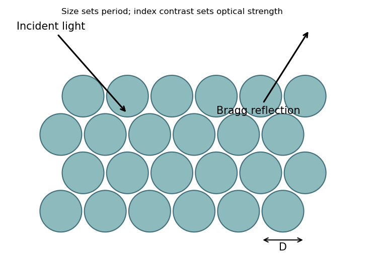
This connects sphere-level geometry and material response to collective periodic optical behaviour. The Bragg reflection estimate does not establish a complete three-dimensional photonic band gap.
Relevant interactions include van der Waals attraction, electrostatic attraction or screened repulsion, hydrogen bonding, and hydrophobic/solvophobic association. Coordination bonding, magnetic dipole interactions and capillary forces can also organize suitable building blocks. Entropic effects, including depletion attraction and packing entropy, can drive ordering even without a new chemical bond. Which contribution favours assembly depends on solvent, temperature, concentration and surface chemistry; the complete balance is a free-energy change, not a requirement that every interaction be attractive.
Self-assembly is organization of interacting building blocks into a larger structure without individually placing every component. Static self-assembly approaches an equilibrium free-energy minimum under fixed conditions; a resulting structure may subsequently become kinetically trapped. Dynamic self-assembly maintains a nonequilibrium organized state through continuing energy or matter throughput and dissipation, and can change or disappear when that drive is removed.
For nanofabrication, parallel assembly of many small components can generate fine periodicity, hierarchical structures and adaptive or self-repairing arrangements with limited direct patterning. Building-block chemistry encodes interactions. However, access to a desired morphology depends on kinetics and competing states; assembly does not automatically eliminate defects or provide arbitrary device geometry.
With the left reservoir at and the right at zero, let the pore run from to . In the stated idealization the reservoir potentials are flat, the pore potential is , and its electric field is , directed from high to low potential. The field is zero in the ideal equipotential reservoirs; real access regions would round these abrupt boundaries.
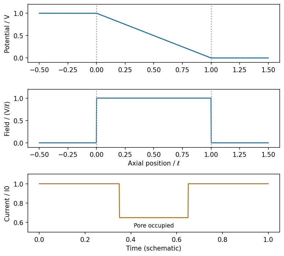
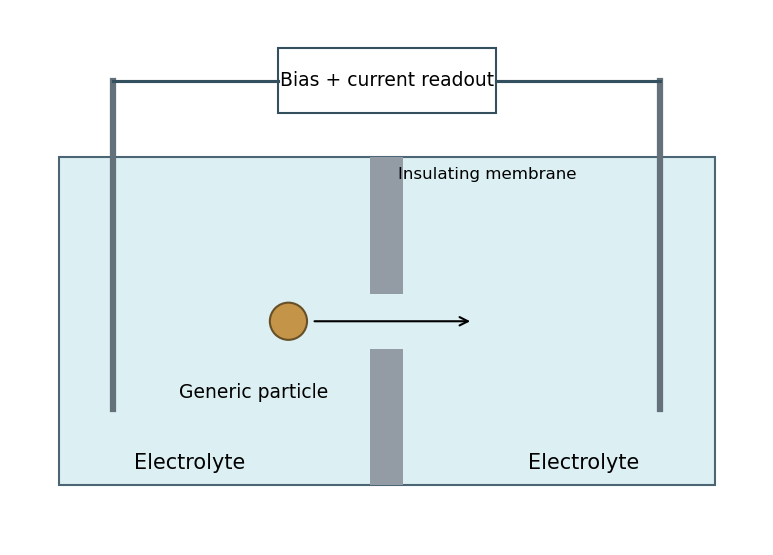
Ideal potential, field and current blockade for a generic insulating particle crossing a uniform pore
. Source. Details. For constant-speed passage and an approximately position-independent in-pore obstruction, the current has a rectangular downward pulse from to during occupation. Entry, exit, filtering and nonuniform fields round real pulses. This describes a physical particle signal without inferring any biological identity or charge.
Ignoring access effects and wall charge, the cylindrical conducting liquid hasThe corresponding conductance is approximately . A charged surface can contribute mobile counterions and change this estimate. Surface conduction is important when its conductance is comparable with the bulk contribution: for surface conductance , their ratio in a cylinder is , twice the Dukhin number convention . Double-layer overlap, when the Debye length is comparable with the pore radius, is another warning that uniform bulk conductivity is inadequate. No surface-charge or ionic-strength data are supplied to quantify those corrections.
In generic resistive-pulse sensing, two electrolyte reservoirs are connected through a small aperture. Electrodes apply a bias and a low-noise current amplifier records the pore current. Passage of a weakly charged insulating particle excludes conducting liquid, usually increasing resistance and giving a transient current decrease at fixed voltage. Pulse amplitude, duration and event rate contain size-, transport- and concentration-dependent information, subject to calibration.
Advantages include label-free single-particle counting, electrical readout and small active volume. Limitations include clogging, electrode/pore noise, finite bandwidth, uncertain particle trajectories and surface-conduction effects; a pulse is not intrinsically chemically specific. Strong particle charge or concentration polarization can complicate, or even reverse, the simple blockade signal. The schematic below uses only generic nonbiological particle transport.
The intended double-barrier resonant-tunnelling diode has a bias-dependent well level. Initially increasing bias can bring a quasi-bound level into alignment with available occupied emitter states, sharply increasing current. At larger bias the resonant level moves out of the effective injection window, for example below the emitter conduction-band edge, so resonant transmission and current decrease despite increasing voltage. This produces a peak-to-valley interval with . Further bias can increase nonresonant or higher-level current again.
The right panel of the preceding figure is a qualitative example. The device can supply small-signal negative differential conductance to an appropriate oscillator circuit while its current and voltage remain positive. A bias-independent transmission function alone does not guarantee NDR: the voltage-dependent potential profile, contacts and carrier supply must be included. The source's reference to part (ii) appears to point to the earlier barrier matching; the resonant device mechanism uses the added barrier of part (iii).
Between two barriers, region III becomes a finite intermediate well containing both right- and left-moving oscillatory components, . Repeated reflection produces standing-wave-like enhancement and quasi-bound levels with finite escape lifetimes. At resonant energies, the multiple transmitted amplitudes add constructively: an ideal symmetric lossless pair can have transmission approaching unity even when a single barrier transmits poorly. Away from resonance the pair strongly suppresses transmission.
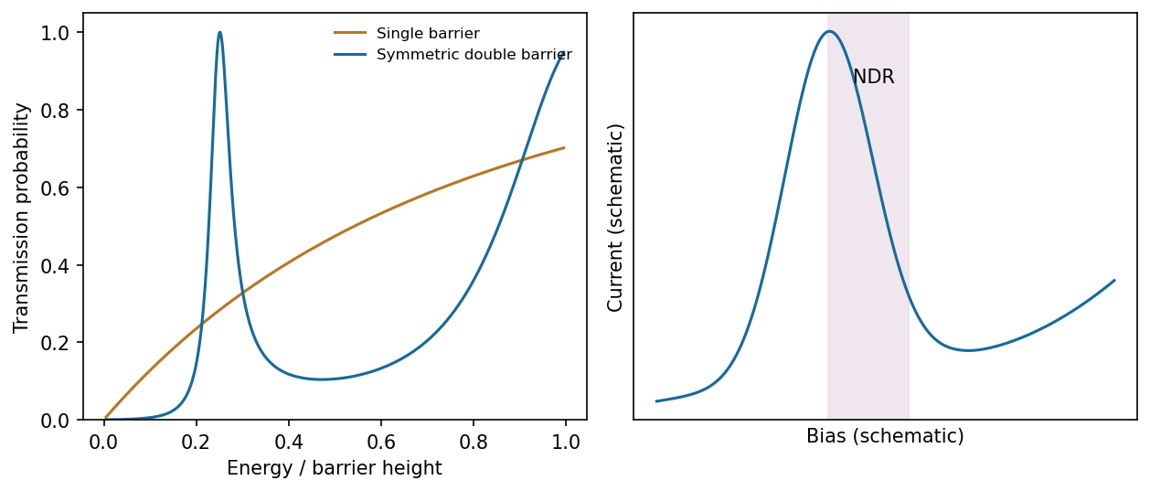
Calculated single- and double-barrier transmission and a separate qualitative resonant-tunnelling current-voltage characteristic
. Source. Details. A useful phase condition is , where is the intermediate-well width and the reflection phases account for penetration into the barriers. The printed figure starts the second barrier at , so its well width is ; if the prose's second-barrier position is used instead, the width is . The resonance argument is unchanged once that geometrical convention is fixed.
For a finite potential step and constant mass, and are continuous. A finite jump of would require a delta-function contribution in the integrated equation, while a jump of would be still more singular. Matching the preceding amplitudes givesThe transmission probability is because the incident and transmitted regions have equal wave vector and mass; in unequal leads a velocity ratio is also required. These matching conditions do not apply unmodified to infinite walls, delta barriers or mass discontinuities.
Take and equal electron mass in all regions. Define and . ThenThere is no wave incident from the far right. Region I contains oscillatory incident and reflected waves; region II is evanescent, with real exponentials rather than propagating plane waves. Both exponential terms are allowed in a finite barrier; deleting the growing term before boundary matching is generally incorrect. A complex superposition in the barrier can carry a nonzero conserved tunnelling current.
For a tube, . A cut normal to its axis crosses ten axial load-bearing C-C bonds in the ideal unstrained honeycomb geometry. Assuming equal load sharing and simultaneous failure at per bond,The graphene areal mass is , giving linear mass densitysince the tex unit has . Thus the ideal carbon nanotube tenacity isThis neglects vacancies, curvature-induced changes in bond strength, thermal activation, imperfect load sharing and structural relaxation at failure. An aligned macroscopic fibre is a network of finite tubes or bundles: sliding, weak intertube shear transfer, imperfect alignment, defects and unequal load participation limit its strength. The nominal fibre diameter alone does not turn it into one defect-free covalent cylinder, explaining why a value near can be much lower than this ideal single-tube estimate.
The real-space carbon honeycomb has two atoms in a primitive cell of its triangular Bravais lattice. The reciprocal lattice is also triangular, and its Wigner-Seitz cell is a hexagonal first Brillouin zone. With a consistent orientation convention, the reciprocal-zone hexagon is rotated by relative to a real-space carbon-ring hexagon; reciprocal lengths scale inversely with the direct lattice spacing.
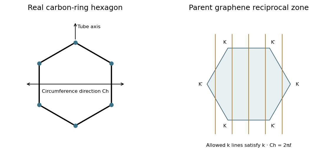


Rolling into a tube imposes , leaving parallel allowed lines in graphene's two-dimensional reciprocal space. They run along the tube-axis direction, perpendicular to the circumferential wrapping vector. The nanotube's actual one-dimensional Brillouin zone is an interval of axial wave vectors with period , where is its axial translation. The parent hexagon is therefore a zone-folding construction, not a literal two-dimensional Brillouin zone for the finished one-dimensional tube.
There are unlisted articles, also show them or only show them.