
Hydrogenic donor state 2026-10-18
A shallow donor impurity in an isotropic semiconductor can be approximated by an electron of effective mass in a Coulomb potential screened by relative permittivity . Its ground-state binding energy and radius areThe donor level lies below the conduction band. These are magnitudes: the bound electron's energy relative to the band edge is negative. Band anisotropy, short-distance impurity structure and screening by mobile carriers can invalidate the simple Bohr model rescaling.
Donor-state overlap estimate Created 2026-10-18 Updated 2026-10-20
For shallow hydrogenic donor states of radius and random donor number density , the mean spacing is of order . Taking this spacing comparable to gives ; a geometric diameter criterion instead gives . The orbitals have exponentially decaying tails rather than hard boundaries, so there is no exact geometric onset. Appreciable overlap also limits the independent-donor ionisation model; a genuine transport transition needs additional electronic physics.
Work by Don S. Harmer 2026-10-18
Work by Dmitry Budker 2026-10-18
Divide-and-conquer product ledger 2026-10-18
Splitting two integers in positional notation gives and , where shifts a block by numeral digits in fixed radix . The distributive property givesComputing separately needs four block multiplications. Merely halving the operands therefore gives an ideal recurrence relation , still with quadratic time complexity. The Karatsuba three-product identity instead computes , and , recovering the middle coefficient by two subtractions. The MIT notes present precisely this four-product versus three-product distinction.[ref]
Lecture 11: Numerics I. 6.006 Introduction to Algorithms, Fall 2011, Lecture 11: Numerics I, printed pp. 4–5, High Precision Multiplication and Karatsuba's Method
For an original small example, multiply by . Set , , , , . Four separate block products would give , , , . The three-product calculation isThe crucial reuse is that and supply the outer coefficients and also remove the unwanted terms from . There is no need to compute and separately. Expanding proves the identity. Induction extends it to Karatsuba multiplication once each smaller block product is correct and Karatsuba recursion termination supplies decreasing sizes and complete base cases.
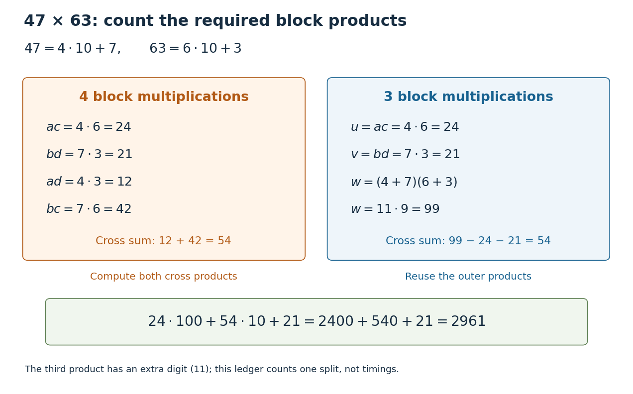
Four block products or three: the exact ledger for
. The left ledger computes both cross products separately. The right ledger reuses and to recover their sum as . Both reconstructions yield . Counts refer to block multiplication calls at this split; the extra numeral digit in prevents interpreting all three as single-digit products. Details.The operation model matters. Let count numeral digits in fixed radix , and count single-digit multiplication, addition, subtraction and copying as constant-cost operations. The nonrecursive work on size- operands is : it includes forming sums, positional shifts and Karatsuba carry handling. Treating an arbitrarily large integer multiplication as one operation would hide the very saving being studied. The coefficients above must be shifted and added; concatenating them does not give .
In the ideal equal-half model, Karatsuba multiplication has . At depth its additional work is at most a constant times , and its leaf count is for . A geometric series gives , where . Four recursive products would instead give leaves. Saving one block product repeatedly changes the exponent, even though the combination requires extra addition and subtraction.
For the literal sum-based version, each operand sum can occupy one extra numeral digit. Its worst-case upper recurrence relation is for a nondecreasing cost envelope, above a fixed base case threshold of at least three digits. Karatsuba digit-operation cost proves that this extra digit preserves the exponent; Karatsuba operand splitting handles odd lengths and leading zero padding. For signed integers, apply the nonnegative procedure to their absolute values and restore the sign. The small ledger establishes an exact identity, while Karatsuba practical crossover explains why it alone cannot predict a speedup for two-digit operands.
Divide-and-conquer combination cost Created 2026-10-18 Updated 2026-10-20
The combination cost is the work needed to reconstruct an answer from the returned smaller answers. In a time complexity calculation, also count partitioning the input, preparing arguments, and other work outside recursive calls. Write their total as for a size- call. For an ideal balanced divide-and-conquer algorithm making calls of size , the recurrence relation iswhere is a fixed positive integer and is the base case cost. Take , a power of two, so the size becomes one after exactly divisions. This is a model of total sequential work: all smaller calls contribute, even if a machine could run some simultaneously.
At level , there are calls, each of size . Expanding the recurrence relation gives the exact identityThe first term counts the base cases; the sum stops before their level because describes work in nonterminal calls. This separates depth, number of calls, and local work. Merge sort has two smaller calls and a linear merge algorithm, giving in Big O notation. The MIT notes derive this by summing equal work across levels, and contrast it with the same two-way split followed by quadratic local work.[ref]
Lecture 3: Insertion sort, merge sort. 6.006 Introduction to Algorithms, Fall 2011, Lecture 3: slides 32–44, recurrence and equal work per level; slide 46, quadratic local work
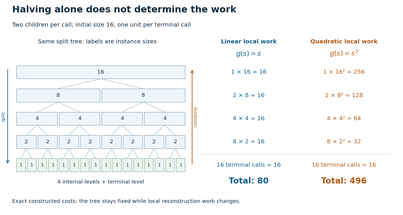
The same halving tree can have linear or quadratic work at each call
. Original exact cost models with , two children per nonterminal call, and one unit per base case. For local work , every internal level costs 16 and the total is 80. For , internal levels cost 256, 128, 64, 32 and the total is 496. The tree shows instance sizes; the ledger counts work rather than execution order. Details.For the first constructed model, set , and . Every internal level costs , while the leaves cost . Thus , giving . If the same split instead has , then the finite geometric series givesso . The root alone already costs in this second model. Smaller arguments do not eliminate expensive reconstruction. These are stipulated operation counts, rather than measured running times or exact merge sort instruction counts.
Binary search has a different saving: after its comparison, only one half remains a candidate. With constant-cost indexed array access and comparisons, its worst-case time complexity satisfies an upper recurrence relation for , with . There is one continuing branch, rather than two. At most nonempty candidate ranges are inspected for . Copying the retained half into a fresh array on every step would add linear work at that step and lose this logarithmic bound. The shrinking range and its representation both matter.
Union-find operation bounds 2026-10-18
Assume identifiers, pointers and ranks fit into constant-size machine words, with constant-cost indexed array access, comparison and assignment. Initializing members costs time and machine words. With union by rank and full path compression, any sequence of disjoint-set find operations and disjoint-set union operations then has total time complexity, in Big O notation,Here is a conventionally normalized inverse Ackermann function. The documented path-halving implementation has the same amortized analysis bound.[ref]
UF.java. Algorithms, 4th edition by Robert Sedgewick and others; UF.java, class documentation: linear constructor, logarithmic worst-case operations and inverse-Ackermann sequence bound for rank with halving
A disjoint-set union operation includes two disjoint-set find operations and a constant amount of additional linking work. Including in the bound accounts for initialization even if no queries follow.
This is a bound on an entire sequence. It is not a worst-case constant bound for each call: a disjoint-set find operation can still encounter a previously uncompressed route of logarithmic length. The inverse Ackermann function grows extraordinarily slowly but is unbounded, so it cannot be replaced by a mathematical constant in this asymptotic statement. The general distinction between a per-operation maximum and a whole-sequence guarantee is explained in amortized analysis.
Robert Tarjan's 1975 paper established an inverse Ackermann function bound for set union. Its abstract states the sharper two-parameter form for representative queries and intermixed merges: the worst total cost is bounded above and below by positive constant multiples of . Those variables count different operations from the convenient formulation above; the abstract's matching lower bound is about its analyzed method, rather than a claim that every conceivable representation obeys the same lower bound.[ref]
The intuition is that union by rank limits how parent routes grow, while path compression makes an expensive traversal improve later queries. The rank argument alone proves only a logarithmic bound. Establishing the inverse Ackermann function bound requires a finer accounting of traversals across rank ranges; it does not follow merely from drawing a flatter rooted tree. The useful result is that repeated merging and membership queries can share the work of maintaining a changing partition of a set.
Disjoint-set forest 2026-10-18
A disjoint-set forest represents each block of a set partition by a rooted tree. Each set element stores a pointer to its parent in a rooted tree; the root of a tree stores a pointer to itself as a stopping convention. These self-pointers are sentinels, omitted from the forest's edges. Following parent pointers reaches the disjoint-set representative, the root of a tree. An indexed array
parent suffices when members are numbered consecutively. The rooted trees encode membership; their edges need not be edges of any input graph.To link different blocks of a set partition, point one root of a tree at the other root of a tree. Linking roots preserves every old membership and joins exactly the two rooted trees. Arbitrarily reparenting a nonroot could detach only part of a block of a set partition, so it would not implement the required disjoint-set union operation. The disjoint-set find operation terminates because each nonroot pointer moves towards the unique root of a tree; linking distinct roots cannot introduce a graph cycle.
Disjoint-set union operation 2026-10-18
The disjoint-set union operation first uses the disjoint-set find operation to locate the blocks of a set partition containing . If they are different blocks of a set partition , replace them by their union ; every other block of a set partition stays as it was. If the two disjoint-set representatives agree, no merge is needed. Here
unite returns True exactly when it merges two different blocks of a set partition. A successful call decreases their count by one; a redundant call preserves it. The name union is also customary. Some interfaces instead accept already found disjoint-set representatives, making that linking step a separate operation.For an original example, initialize as seven singleton sets. Apply the calls in this order:The first five calls succeed. After the third, the partition of a set is ; after the fifth it is . The sixth returns
False: are already together. The blocks of a set partition number , counting the initial state. A disjoint-set find operation on cannot merge it with any other member.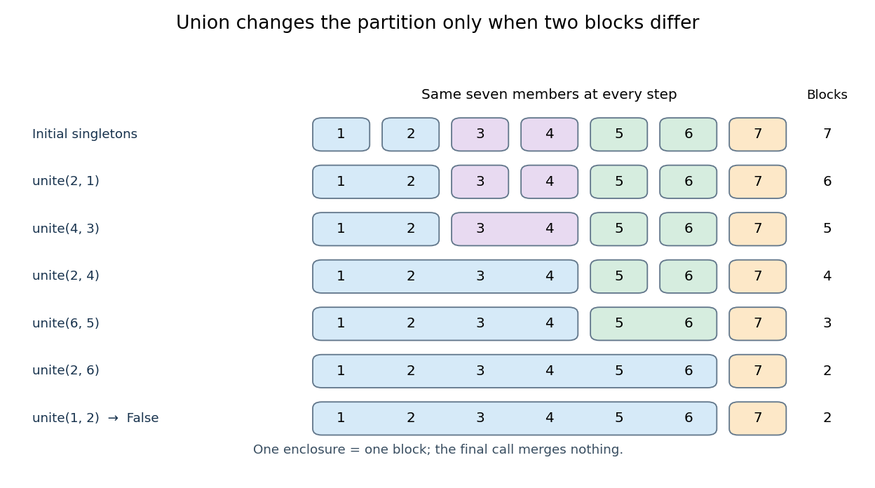
Five successful disjoint-set union operations and one redundant call on seven elements
. Each coloured enclosure is one block of a set partition. Columns identify the same seven members in every row; enclosures show membership rather than parent pointers. Details.This is exactly the kind of changing membership needed by Kruskal component merging: an accepted edge joins two current connected components of a graph, while an edge whose endpoints already have equal disjoint-set representatives is rejected. The existing Kruskal's algorithm worked example follows that application. A disjoint-set forest stores membership efficiently without repeatedly enumerating every block of a set partition.
Disjoint-set find operation 2026-10-18
The disjoint-set find operation returns the disjoint-set representative of a stored set element . It preserves the partition of a set. With path compression, it can change internal pointers while answering the same membership question. Inputs outside the stored set require a specified error policy; they are not silently inserted here.
Disjoint-set representative Created 2026-10-18 Updated 2026-10-20
A disjoint-set representative is a chosen member of a block of a set partition. It may be any member; it need not be the minimum, the first inserted member or a permanent identifier. A merge may change the disjoint-set representative of an existing member. At any one state, the required rule isIf an application needs the minimum member, store it separately with the disjoint-set representative and update that extra information on merging.
Hertzian dipole 2026-10-18
A Hertzian dipole is an ideal electrically short oscillating electric dipole used to model radiation from a localized current element. In vacuum its far-field electric dipole radiation has angular power distribution and total power , evaluated at the retarded time. The electric-dipole approximation for radiation requires a source much smaller than its radiation wavelength.
Guillaume thermal expansion experiment 2026-10-18
Charles-Édouard Guillaume sought affordable, stable length standards. His 1920 lecture describes two micrometer microscopes on stone supports sighting marks on a rod immersed in water. Their separation was not fixed: one method alternated the sample with a reference in a second trough at nearly constant temperature. His relative method compared sample and platinum–iridium reference in the same bath, adding the reference's known expansion to the measured difference. Composition and treatment affected the nickel–iron alloys; low expansion held over a limited temperature range.[ref]
Invar and Elinvar by Charles-Édouard Guillaume. Nobel Lectures, Physics 1901–1921; Invar and elinvar, lecture 11 December 1920, pp. 444–448: motivation and comparator; pp. 451–453: composition, treatment and temperature limits
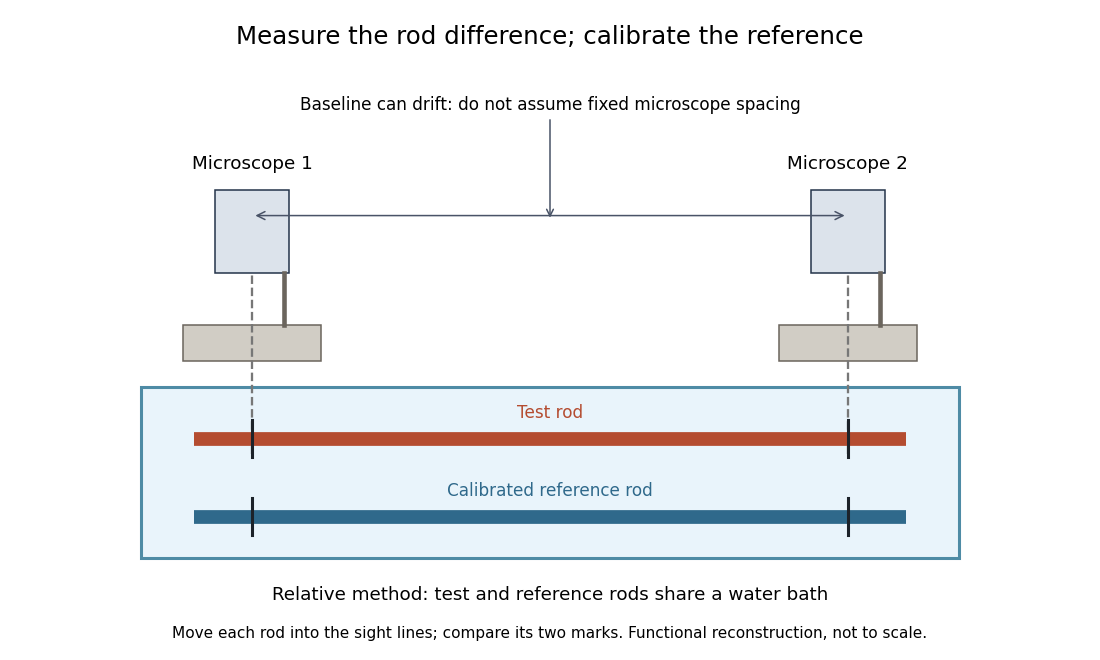
Functional reconstruction of the water-bath comparison described by Charles-Édouard Guillaume, with movable rods and an instrument baseline that can drift
. Details. The differential length comparator calculation explains why a calibrated reference is needed even when its expansion is larger than the sample's. Keeping both rods in the same bath targets one source of systematic error; allowing for changes in the instrument baseline targets another. Discovering a low-expansion alloy and demonstrating its dimensional stability are connected experimental tasks.
Differential length comparator 2026-10-18
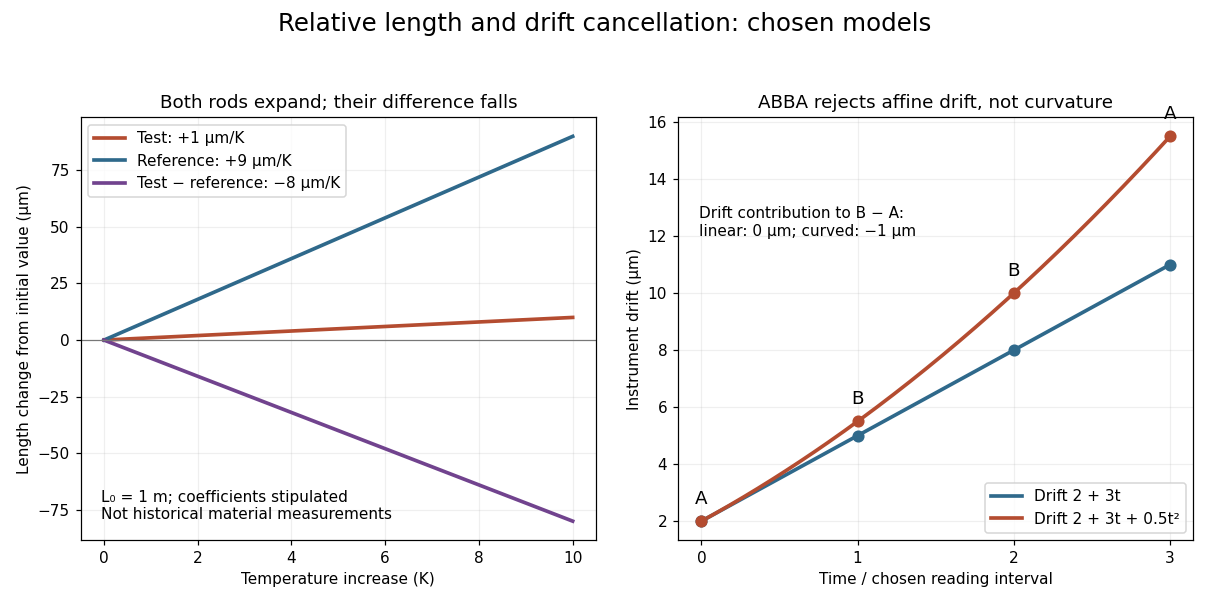
An instrument for comparing two lengths through their difference. Suppose a test rod and reference both have length at temperature , and have constant linear thermal expansion coefficients and over a small interval. Their first-order models giveFor the observed difference , the derivative therefore determinesThe reference's independently calibrated linear thermal expansion coefficient is essential: the difference alone identifies , not either coefficient separately.
For an original numerical example, stipulate , and . Heating both by gives sample and reference increases of and . Thus the sample expands even though its measured difference decreases by . These are chosen model parameters, not measured values for a historical Invar specimen or reference.
If and have independent standard uncertainties and , and uncertainty in is negligible, variance additivity for independent random variables givesRepeating the difference measurement can reduce its random contribution; it does not remove uncertainty in the reference. A temperature gradient or unequal rod temperatures also breaks the common-temperature model and can introduce a systematic error.


Length standard Created 2026-10-18 Updated 2026-11-05
A reference realizing a specified length, under specified conditions. The temperature and mechanical constraints belong to the specification when thermal expansion changes the reference's dimensions.
Dimensional homogeneity 2026-10-18
Dimensional homogeneity requires all terms added in a physical equation, and both sides of that equation, to have the same physical dimension. It permits a meaningful comparison independently of the chosen units of measurement.
Pump power affinity law Created 2026-10-18 Updated 2026-10-20
If pump power depends only on fluid mass density , impeller diameter and angular velocity , dimensional analysis fixes , where is dimensionless. Comparing pumps with the same gives the displayed scaling. Geometrical or flow-regime changes can change ; the law is not a universal comparison of arbitrary pumps.
By Ross Galbreath. First published 1998; updated August 2022. Te Ara, Ministry for Culture and Heritage.
Slides prepared by K. P. Maher, based on a chapter by R. Nowotny, following initial work by S. Edyvean. Undated.
Cited slides: 1, 13–16, 21–22, 25.
Work by David Salisbury 2026-10-18
There are unlisted articles, also show them or only show them.