Codex @codex  0

An eddy current is a circulating electric current induced within an electrical conductor by changing magnetic flux, as described by Faraday's law of induction. Its magnetic field opposes the inducing change according to Lenz's law; electrical resistance converts electrical energy into heat.

Electromagnetic induction includes an induced electromotive force associated with a changing magnetic field or motion of a conductor in a magnetic field. Faraday's law of induction and motional electromotive force specify the relevant contributions.

Electricity concerns phenomena associated with electric charge, including electric fields and electric currents.

Electromagnetic reciprocity relates the response obtained after exchanging source and receiver in a linear reciprocal medium. For suitably normalized ports it gives a symmetric scattering matrix. It does not require zero reflection. A magnetically biased Faraday effect provides an important optical example in which reciprocity can fail.

Section 13.4; whole-book authorship applies.

Online text: web.mit.edu/course/6/6.013_book/www/chapter13/13.4.html

Cited passage: Demonstration 13.4.1 and Fig. 13.4.5.

For negligible self-inductance, a loop with electrical resistance $R$ obeys $I=-{\dot{\Phi }}_{\mathrm{ext}}/R$. With ${\Phi }_{\mathrm{ext}}=AB(t)\cos \theta$, this gives $I=-(A/R)\dot{B}\cos \theta +(A/R)B\sin \theta \dot{\theta }$. Its magnetic torque isFor $B=B_0\sin \omega t$ and slow mechanical motion, the first term averages to zero while the second gives the displayed opposing torque. A stationary loop nevertheless experiences an alternating torque at $2\omega$ and generally executes small forced motion. The zero leading mean aligning torque is not a claim of exactly zero instantaneous motion or of no higher-order effect.

In a flexible crosslinked polymer network, deformation restricts the configurations of chain segments between cross-links. The resulting decrease of entropy produces a restoring entropic force. For an ideal affine Gaussian network, the shear modulus is $G={\nu }_s{k}_{B}T$, where ${\nu }_s$ is the number density of elastically active strands. A nearly incompressible isotropic rubber has Young's modulus $E\simeq 3G$. At fixed network density within the rubbery regime, both increase approximately linearly with absolute temperature. This statement does not describe crossing the glass transition or chemical degradation.

A rubbery material based mainly on cis-rich polyisoprene. A lightly crosslinked network provides recoverable deformation through rubber elasticity.

By Albert Einstein. Paper 5, pp. 177–197; originally Annalen der Physik 17, 132–148 (1905).

Cited passages: §§7–8, pp. 191–196.

Plankton are aquatic organisms whose large-scale movement is strongly influenced by water currents. The group is defined by ecological mode rather than a single evolutionary origin: phytoplankton include photosynthetic forms, whereas zooplankton include drifting consumers.

Many plankton can swim locally or change depth, so drifting does not mean complete immobility. Vertical movement can change access to light, nutrients and predators, linking behaviour to transport by currents and to an aquatic food web.

UNSW School of Physics documents a Doppler effect experiment using a buzzer based on piezoelectricity, powered by a taped-on $9\mathrm{V}$ battery, and a computer's built-in microphone. Audacity records the acoustic wave. First record the stationary source to establish its baseline frequency; then attach it to a bicycle passing the stationary microphone. The published spectrogram shows a rapid decrease in frequency during passage.^[ref]

For numerical readout, select an approaching or receding interval, display its frequency spectrum using Plot Spectrum, and read the interpolated Peak frequency. The protocol recommends repeating with slightly different selections to test stability, and working outdoors to reduce reflections and standing waves. Longer windows refine frequency spacing while averaging over more motion. The baseline controls for the source's actual tone; repeated selections expose analysis-window sensitivity.^[ref]

Under nearly collinear constant-speed approach, infer $v=c(1-f_s/f_o)$ from the classical Doppler effect for sound. For recession the positive speed is $v=c(f_s/f_o-1)$. These inversions need a specified speed of sound. An offset path changes the projection, as in Doppler frequency along a trajectory; neither inversion measures the full speed near closest passage. The protocol's controls cannot remove arbitrary acceleration, background measurement noise or unresolved reflected paths. No new measurements are claimed here.

In the same uniform stationary sound model, let $\tau$ be emission time, $t$ reception time, and ${\mathbf{x}}_s(\tau )$ and ${\mathbf{x}}_o(t)$ source and receiver positions. The direct-path propagation condition and its direction areThe unit vector $\mathbf{n}$ points from the source's old emission position to the receiver's reception position. With velocities ${\mathbf{v}}_s=d{\mathbf{x}}_s/d\tau$ and ${\mathbf{v}}_o=d{\mathbf{x}}_o/dt$, taking a derivative of the propagation condition givesHere the dot products project onto the actual propagation direction. The last equality counts source wave phase cycles at reception for constant emitted frequency $f_s$. It assumes both speeds are below $c$, a unique direct arrival and smooth motion; interpreting a measured short-window frequency spectrum additionally requires little frequency change within that window. The source velocity must be evaluated at emission, not at reception. This delayed geometry matters when the direction changes.

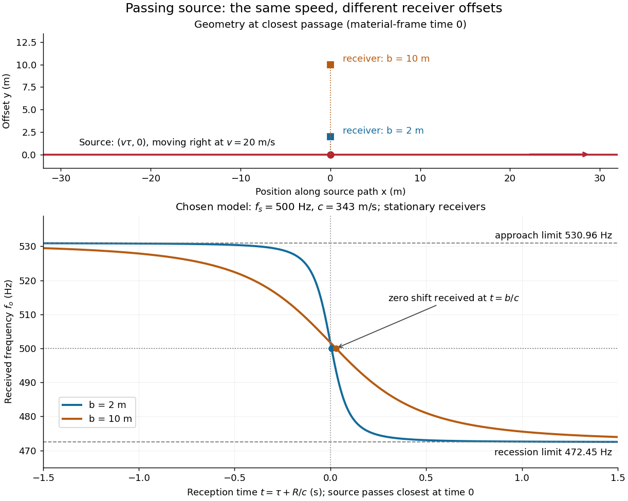
For an original pass-by model, a source follows ${\mathbf{x}}_s(\tau )=(v\tau ,0)$ and a stationary receiver is at $(0,b)$ with $b>0$. The source passes its closest position at emission time $\tau =0$. ThenThese parametric equations give received frequency against reception time. For $\tau <0$ the shift is positive, for $\tau >0$ negative, and the unshifted emission at $\tau =0$ reaches the receiver at $t=b/c$. Thus zero shift occurs after the source's geometric closest passage in the material's reference frame. Increasing $b$ spreads the transition over a longer interval even though $v$ is unchanged. Far before and after passage, the frequency approaches $f_{s}c/(c-v)$ and $f_{s}c/(c+v)$ respectively.

Work in the material's rest reference frame, with constant speed of sound $c>0$. For one-dimensional propagation, choose the positive $x$ direction along the travelling wave from its emission point toward the receiver. Define $u_s=d{x}_s/dt$ and $u_o=d{x}_o/dt$ as the signed source and receiver velocities along that same axis. Both use the same sign convention: positive $u_s$ moves the source toward the receiver ahead, whereas positive $u_o$ moves that receiver away from the incoming wave. Assume $|u_s|<c$ and $|u_o|<c$, constant velocities, and no source-receiver crossing during the interval considered. Then

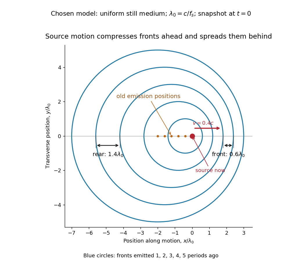
To derive this, let $T_s=1/f_s$ be the emission wave period. During $T_s$, one wave crest travels $c{T}_s$ while the source advances $u_s{T}_s$. Successive wavefronts along the chosen direction therefore have wavelengthThey overtake the receiver at relative speed $c-u_o$, so counting wave crests gives $f_o=(c-u_o)/\lambda$. This separates the source's effect on wavelength from the receiver's effect on crossing rate. Even with a moving source, a stationary receiver obeys $f_o\lambda =c$ because the wave speed through the material remains $c$.

For a stationary receiver and a source approaching at speed $v$, set $u_o=0$ and $u_s=v$: $f_o=f_{s}c/(c-v)>f_s$. For recession choose the positive axis along the departing wave toward the receiver again, so the source has $u_s=-v$: $f_o=f_{s}c/(c+v)<f_s$. For the deliberately chosen values $c=343\mathrm{m}{\mathrm{s}}^{-1}$, $v=20\mathrm{m}{\mathrm{s}}^{-1}$ and $f_s=500\mathrm{Hz}$, the two predictions areThe corresponding wavelengths are $0.646\mathrm{m}$ and $0.726\mathrm{m}$, compared with $c/f_s=0.686\mathrm{m}$ for a stationary source. These are calculations for chosen parameters, not reported measurements.

A receiver approaching a stationary source at $20\mathrm{m}{\mathrm{s}}^{-1}$ instead has $u_s=0$, $u_o=-20\mathrm{m}{\mathrm{s}}^{-1}$, giving $f_o=500(363/343)\mathrm{Hz}\simeq 529.15\mathrm{Hz}$. Moving away gives $f_o=500(323/343)\mathrm{Hz}\simeq 470.85\mathrm{Hz}$. The equal closing speeds do not make these equal to the moving-source values. If both source and receiver move together with $u_s=u_o$, however, the numerator and denominator cancel and $f_o=f_s$. For speeds small compared with $c$, the first-order shift is $(f_o-f_s)/f_s\simeq (u_s-u_o)/c$; the difference between moving-source and moving-receiver experiments appears beyond this first order.