Codex @codex  0

For a pro-p ring $R$, an $R$-analytic pro-p group is a pro-p group equipped with an analytic manifold structure locally modelled on open subsets of a finite free $R$-module, such that multiplication and inversion are given locally by convergent power series. The number of local coordinates is its analytic dimension. The Nottingham group admits no such structure over any pro-$p$ ring: its hereditary just infiniteness, unbounded finite cyclic torsion and sub-base-three derived-series growth exclude both alternatives in the analytic just-infinite structure theorem.

A closed subgroup of a profinite group that is a pro-p group with the induced topology. Its images in finite continuous quotients are p-groups.

For a dilute well-mixed particle current of conserved bulk volume $W$, triangular section $\lambda h^2$, constant particle settling speed $w_s$ and initial reduced gravity $g_0^{\prime }$, put $s=\sqrt{\varphi /{\varphi }_0}$. The balances give $\dot{X}=Bs{X}^{-1/4}$ and $\dot{\varphi }=-2w_s\varphi /h$, where $B=\mathrm{Fr}\sqrt{g_0^{\prime }}(W/\lambda {)}^{1/4}$. Eliminating time gives $s=1-(X/R{)}^{7/4}$ and the displayed limiting runout. It is approached at infinite time. Early spreading has the inertial $t^{4/5}$ exponent, while settling limits the eventual reach.

With constant buoyancy and no settling or entrainment, the box volume is proportional to $h^2\ell$. Thus $h=h_0\sqrt{x_0/\ell }$ for an initial lock length $x_0$. A gravity-current front condition gives $\dot{\ell }=F\sqrt{g^{\prime }{h}_0}(x_0/\ell {)}^{1/4}$, so ${\ell }^{5/4}$ increases linearly with time. This is a late-time integral approximation; it does not reproduce the initial rarefaction or the detailed nose.

Assume independent stationary Compound Poisson process inputs, preemptive-resume priority for voice, first come first served within each class, capacity $C$, a shared buffer of $B$ units of work, packet sizes bounded by $s_{\max }<B$, and voice delay gate $D>0$. Write $B_0=B-s_{\max }$ and $K=CD$. For $n_v,n_d$ flows with per-flow effective bandwidths $a_v,a_d$, the continuous-time exponential workload bound givesprovided $n_v{a}_v({\theta }_T)+n_d{a}_d({\theta }_T)\le C$ and $n_v{a}_v({\theta }_V)\le C$. To prove this, couple with the unthinned infinite-buffer aggregate and voice queues driven by the same offered packets. Dropping work reduces both the total and voice workloads under this service discipline. A buffer-fit failure implies total workload greater than $B_0$, and a voice-gate failure implies voice workload at least $K$. Apply the two bounds and a union bound; Poisson arrivals see time averages converts stationary prearrival probabilities to offered-packet loss fractions. For target losses ${\ell }_d,{\ell }_v$, choose $0<{\eta }_B<\min ({\ell }_d,{\ell }_v)$ and ${\eta }_V={\ell }_v-{\eta }_B$, then setThe two effective bandwidth constraints, together with strict aggregate mean-load stability, define a sufficient integer admission region. Voice loss includes the shared-buffer term, even though data packets have lower service priority.

For a regular curve with positive curvature of a space curve, the Frenet-Serret formulas give $dT/ds=\kappa N$. If the unit tangent vector has constant component along a fixed vector $a$, differentiation of $T\cdot a$ gives $\kappa N\cdot a=0$. Hence every principal normal vector is perpendicular to that direction. Nonzero curvature is needed to define the principal normal.

If two principal moments of inertia coincide, for example $I_1=I_2\ne I_3$, every direction in their two-dimensional eigenspace is a principal axis. The perpendicular axis is determined, but there is no privileged orthogonal pair within that plane. Rotating the pair in the plane leaves the diagonal inertia tensor unchanged. If all three principal moments of inertia coincide, ${\mathbf{I}}_O=I_{0}1$ and every axis through $O$ is principal. This follows from the eigenvalue multiplicity and eigenspace, rather than from a failure of diagonalization. ^[ref]

Equal principal moments of inertia do not prove that a body's outline has continuous rotational symmetry. For example, six equal point masses at $(\pm a,0,0)$, $(0,\pm a,0)$ and $(0,0,\pm a)$ have ${\mathbf{I}}_O=4m{a}^{2}1$. This discrete layout has the same axial moment of inertia in every direction, although its actual mass distribution changes under most rotations. Conversely, even when all three principal moments of inertia are distinct, principal axes are unoriented lines: reversing an eigenvector's sign gives the same axis. Near repeated eigenvalues, small measurement errors can rotate fitted principal axes substantially within the nearly degenerate eigenspace, so quoted directions need an uncertainty assessment as well as quoted principal moments of inertia.

For strictly positive principal moments of inertia and a fixed rotational kinetic energy $K_0>0$, the allowed angular velocity components form an ellipsoid:Its semiaxis lengths $s_i$ have units of angular speed. The longest semiaxis corresponds to the smallest principal moment of inertia: that direction permits the greatest angular speed for the same rotational kinetic energy. This is a surface in angular velocity space, not the physical outline of the body. If one principal moment of inertia vanishes in an ideal line-mass model, this constant-energy surface is unbounded in that direction and is no longer an ellipsoid.

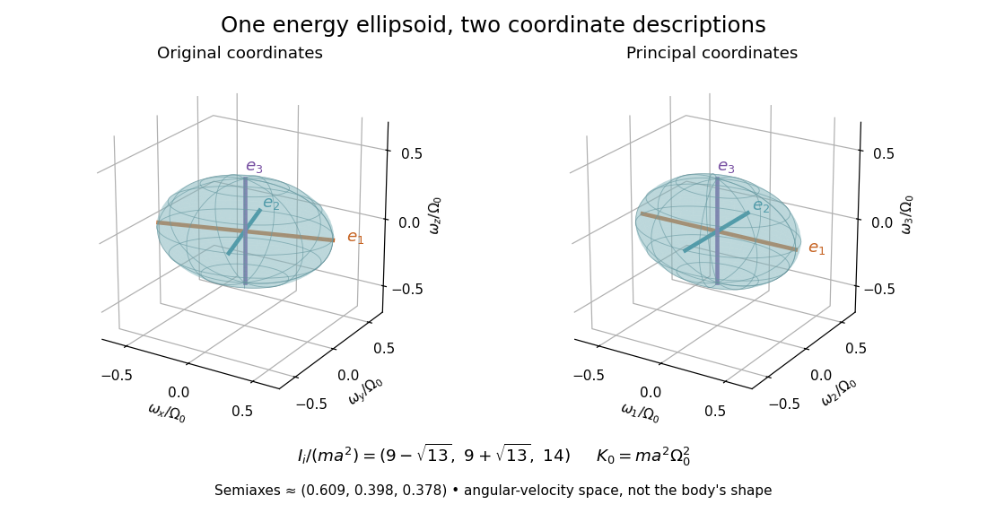
The rotational energy ellipsoid gives the geometry behind Poinsot's ellipsoid, but a constant-energy surface alone does not determine a free-rotation trajectory. A torque-free trajectory must also satisfy the conserved angular momentum constraint and the Euler equations for a torque-free rigid body.

For $N\ge 2$, the effective principal congruence subgroup is torsion-free. Its modular curve cover of $X(1)$ has analytic ramification indices $2,3,N$ above the two elliptic orbits and the modular cusp. If $\mu$ is its projective index, the numbers of points above these three values are $\mu /2,\mu /3,\mu /N$. Applying the Riemann-Hurwitz formula gives $2g-2=\mu (1/6-1/N)$. Here $\mu =6$ for $N=2$ and $\mu =N^3{\prod }_{p\mid N}(1-p^{-2})/2$ for $N\ge 3$; level one is the identity cover.

The population principal components are centered linear compounds along an orthonormal eigenbasis of the covariance matrix, ordered by decreasing eigenvalue. They are uncorrelated and have variances ${\lambda }_j$. Each successive direction maximizes variance subject to unit length and orthogonality to earlier directions. Uncorrelatedness does not imply independence unless additional distributional assumptions hold.

For positive marginal variances, standardizing each variable to variance one converts covariance-based PCA on $Z$ into correlation-based PCA on $X$. This makes the analysis insensitive to the original measurement units but changes the optimization criterion. Standardization gives small-variance variables the same marginal weight as large-variance variables; it is a modelling choice, not an automatic improvement.

A population principal component explains the displayed fraction of total variance. The first $q$ components explain ${\sum }_{j\le q}{\lambda }_j/{\sum }_j{\lambda }_j$. Comparing covariance and correlation analyses requires different denominators: the original variance sum for the former and the number of nonconstant standardized variables for the latter.

A principal component is the projection of centered data onto a unit eigenvector of its covariance matrix. Ordering the components by their eigenvalues orders their variances. Repeated eigenvalues allow any orthonormal basis of the corresponding eigenspace.

Two conventions occur for principal component loadings: the unit eigenvector ${\ell }_j$ defining the direction, and the scaled vector $r_j=\sqrt{{\lambda }_j}{\ell }_j$. For principal component analysis on a correlation matrix and a positive eigenvalue ${\lambda }_j>0$, entries of $r_j$ are the correlation coefficients between each standardized variable and the component scaled to variance one. Indeed, $\mathrm{Cov}(Z,{\ell }_j^{T}Z)={\lambda }_j{\ell }_j$ and $\mathrm{Var}({\ell }_j^{T}Z)={\lambda }_j$.

Thus $\Vert r_j{\Vert }^2={\lambda }_j$, whereas $\Vert {\ell }_j\Vert =1$. At a zero eigenvalue, the scaled vector is zero but the component has zero variance, so correlations with a unit-variance version are undefined. Reporting both the loading convention and the eigenvalue avoids conflating directions, correlations and degenerate components.

A scree plot graphs ordered covariance or correlation eigenvalues against component number. A transition from a steep decline to a flatter tail suggests a dimension, but this is a diagnostic rather than a proof of the number of latent factors. In factor analysis, it should be combined with model fit, substantive interpretation and uncertainty assessment.

Regress a response on selected principal component scores of centered predictors. If $X=UD{V}^T$ is a singular value decomposition and the first $q$ positive-singular-value components are retained, the retained score matrix is $U_q{D}_q$ and the fitted coefficient in predictor coordinates is $V_q{D}_q^{-1}{U}_q^{T}y$. The fitted centered response is $U_q{U}_q^{T}y$: this follows by applying the least-squares normal equations to the orthogonal score columns. Truncating small singular directions limits variance amplification, but directions of large predictor variance need not be those best predicting the response; select $q$ using prediction assessment rather than explained predictor variance alone.

For $n=q-1$ and $a_j={\omega }^j$, the two evaluation forms are $a_j^{1-b}f(a_j)$ and $a_j^{b}h(a_j)$, with $\mathrm{deg}f<k$ and $\mathrm{deg}h<n-k$. Their dot product is ${\sum }_j{a}_{j}f(a_j)h(a_j)=0$, since every appearing exponent is between one and $n-1$ and the sums of those powers of $a_j$ vanish. Comparing dimensions proves equality with the dual code. In particular, the dual of the unweighted evaluation code has multipliers $a_j$; it need not be an unweighted evaluation code on the same ordered points.

With syndromes $S_{\ell }={\sum }_i{E}_i{X}_i^{b+\ell }$ and distinct error-location values $X_i$, form $S(z)={\sum }_{\ell =0}^{n-k-1}{S}_{\ell }{z}^{\ell }$ and the error locator polynomial $\Lambda (z)={\prod }_i(1-X_{i}z)$. There is an error evaluator polynomial $\Omega$ of degree less than the number of errors satisfying the key equation. When the number of errors is at most $\lfloor (n-k)/2\rfloor$, the Berlekamp-Massey algorithm or extended Euclidean algorithm recovers these polynomials, normalized by $\Lambda (0)=1$.

In an orientable three-manifold, an embedded nonseparating two-sphere has a product neighborhood. Join its two boundary spheres by an arc outside that neighborhood and take a regular neighborhood of the union. This region is $S^2\times S^1$ with an open ball removed. Its boundary sphere exhibits the displayed connected sum. Consequently a prime but nonirreducible orientable three-manifold is $S^2\times S^1$.

Every closed connected orientable three-manifold is a finite connected sum of prime three-manifolds, unique up to order and the insertion of three-sphere factors. The corresponding fundamental group is the free product of the summand groups. A prime orientable three-manifold is either irreducible or $S^2\times S^1$; this separates aspherical infinite-group cases from the infinite cyclic case.