
Beta number of a partition Created 2026-10-14 Updated 2026-11-05
For a partition padded to rows, its beta numbers are the distinct nonnegative integers . They are its occupied abacus of a partition positions. With exactly the positive row count, they equal the first-column hook lengths; extra zero rows change the representation of the beta set while preserving the partition. Individual beta numbers describe bead positions, whereas the beta set is the collection of all these numbers.
Parallel beta reduction 2026-10-14
Parallel beta reduction permits simultaneous reduction in the body of a lambda abstraction and both sides of an application, together with when and . Variables reduce to themselves. Its capture-avoiding substitution lemma is . Its transitive closure equals ordinary finite beta reduction, while its one-step diamond property yields the Church-Rosser theorem.
Diamond property of a reduction relation 2026-10-14
A reduction relation has the diamond property if and imply a common one-step successor . For relations allowing an identity step, the same definition includes zero-length joins. A finite grid of these diamonds proves confluence of . Ordinary one-step beta reduction fails this property because contracting before duplication can save two separate contractions.
Commutation allows exchanging the factors at their existing arguments; it does not allow exchanging their arguments while retaining the same pole sign. With the displayed convention, differentiation produces and . These signs are essential for the conformal weights and central charge of a commuting beta-gamma system.
Using the radial-ordering sign in commuting beta-gamma contractions, single contractions give and the corresponding weight for . Put and . Their double-contraction coefficients in are respectively . The fourth-order pole of is therefore , which equals . There is no anticommuting Wick sign.
Beta-binomial distribution Created 2026-10-14 Updated 2026-10-20
Mix a binomial distribution with a beta distribution for its success probability: and . Integrating their densities gives the displayed mass for . Its expectation is , and its variance is . It is the posterior predictive distribution for repeated Bernoulli trials after a beta-prior update.
Couple and from , with . Suppose their finite lifetimes end at zero and . Their difference is positive and has derivative , so . For , the Itô formula givesThe normalized scale function of a one-dimensional diffusion is a bounded local martingale. Its finite quadratic variation and the divergent clock force on simultaneous extinction; on strict extinction . Its terminal value is therefore the strict-extinction indicator, proving the formula by optional sampling theorem. For SLE boundary images, ; this compares strict and simultaneous boundary swallowing times for .
Three-dimensional Bessel process 2026-10-14
The radial part of three-dimensional Brownian motion started away from the origin is a Bessel process of dimension three. The radial Laplacian is , so the Itô formula gives the displayed equation. The radial martingale has unit quadratic variation rate and is Brownian motion by the Lévy characterization of Brownian motion. The reciprocal is a local martingale. Stopping it on gives . Letting shows that zero is not hit.
For , the drift is globally Lipschitz and bounded. Solve its equation strongly for the prescribed Brownian motion, and stop at the first hit of . Local uniqueness makes these stopped solutions agree up to the larger threshold; their stopping times increase as the threshold decreases. With , Itô's formula for gives on every finite horizon. Hence the patched lifetime is infinite. Localization away from zero proves pathwise uniqueness of the positive global solution. Uniqueness before a stopping time refers to the stopped solution, not to arbitrary unconstrained continuations afterward.
Oppositely driven Bessel exit probability 2026-10-14
For , couple and from positive , killing each at zero. Their sum has no Brownian term and increases, so simultaneous extinction is impossible. The ratio has time-changed generator . Its scale density is , integrable at both endpoints. Optional stopping of its normalized scale function at the first extinction gives the displayed regularized incomplete beta function. At this is Cardy's formula.
Squared Bessel process 2026-10-14
A squared Bessel process of dimension is a nonnegative continuous solution of the displayed stochastic differential equation. It extends the squared radial part of integer-dimensional Brownian motion to arbitrary nonnegative dimensions. Before hitting zero its square root solves . At dimension zero, a process started at zero remains there. The coefficients are not Lipschitz at zero, so positivity or uniqueness must not be justified by a global Lipschitz theorem.
Two-dimensional Bessel transition law 2026-10-14
A dimension-two Bessel process starting at has the displayed marginal law, where are independent standard normal random variables. Take the norm of a planar Brownian motion starting at . Planar Brownian motion avoids a fixed point, so the norm stays positive; Itô formula gives drift and a martingale term of bracket . The Lévy characterization of Brownian motion identifies that term as its driving Brownian motion. The squared radius divided by has a noncentral chi-squared distribution with two degrees of freedom and noncentrality .
Bessel focal length uncertainty 2026-10-14
For small measurement errors, write . Its partial derivatives and first-order propagation of uncertainty areHere the values are standard deviations used to describe uncertainty, and is the covariance. Independent carrier-reading errors give ; correlated readings require the term . Averaging repeated independent pairs reduces the random component of the uncertainty of the mean, but does not remove calibration or model errors.
As a stipulated uncertainty calculation, let , , and , with all three input errors independent. Then , , and . The result would be with this standard uncertainty in the stipulated thin lens model; these numbers are not a measured uncertainty budget. A small neglected principal-plane separation gives an additional first-order bias , distinct from that random budget.
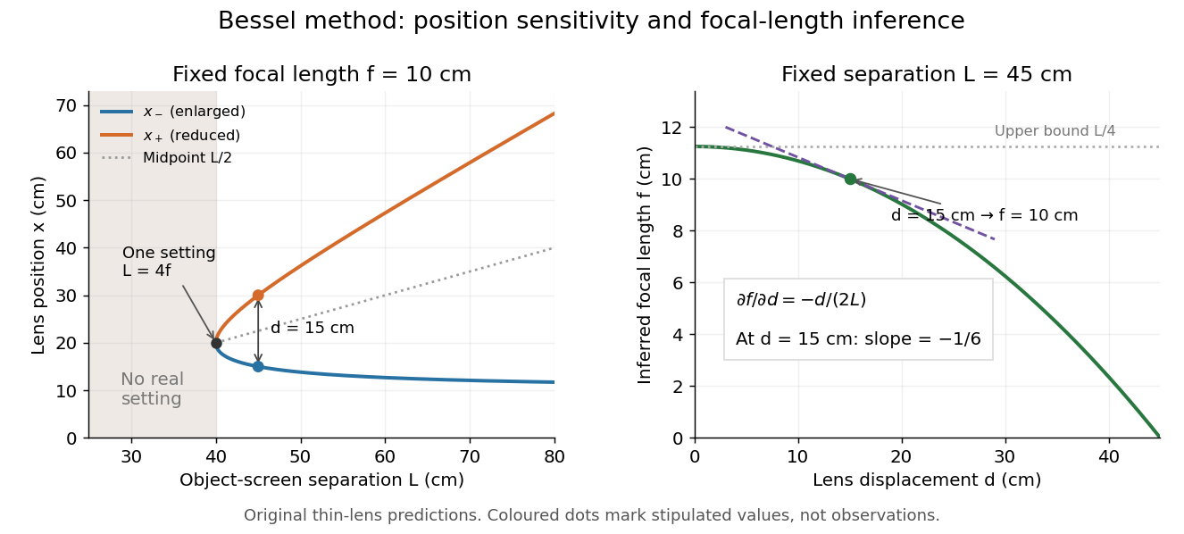
Bessel lens displacement method: merging settings and focal length sensitivity
. Original ideal-model curves. Left: settings versus object-screen separation for fixed ; below there is no real setting on the fixed screen. Right: inferred focal length versus measured displacement at fixed , with its tangent at the stipulated . The curves are predictions, not experimental points. Details.
The two kinds of sensitivity must be distinguished. At fixed focal length,These derivatives diverge as approaches from above: a small change in object-screen spacing strongly changes the separation of the two settings. Yet the inferred focal length's displacement sensitivity tends to zero. That does not make coalescing settings easy to measure. For fixed , define the axial mismatch between the predicted real image and the screen as , for . At a focused setting,Near , moving the optical lens changes this mismatch only weakly, making visual discrimination of the two settings difficult. At the example's settings and , so equal carrier motion produces different axial defocus responses. This is an axial mismatch calculation, not a full prediction of perceived image sharpness.
Choose sufficiently above to separate the two accepted focusing ranges, while retaining both real images on the available screen and rail. There is no universal best : focusing uncertainty itself depends on aperture, transverse magnification, optical aberrations and the target. Close to , the nonnegative measured separation and the quadratic term in also make first-order propagation of uncertainty unreliable if its error is comparable to its value. Repeatability, controls and the principal plane correction determine whether the elegant two-distance formula is an adequate measurement model.
Bessel lens displacement experiment 2026-10-14
KIT's teaching apparatus uses a glass spoke-wheel or test negative as the object, a halogen lamp with an illuminating optical lens, an imaging optical lens, a screen and a triangular rail with a position scale. The illuminating optical lens concentrates the lamp filament's image on the imaging optical lens's centre; translucent paper checks that illumination. This reduces the contribution of peripheral light rays and their spherical aberration. The instructions require fixed object-screen separation exceeding , at least ten displacement measurements, and separate red- and blue-filter measurements to test chromatic aberration.[ref]
Brennweite dünner Linsen by Karlsruhe Institute of Technology, Faculty of Physics teaching laboratory. Karlsruhe Institute of Technology, Brennweite dünner Linsen, Durchführung and Aufgaben 1a and 2: target, illumination check, rail readout, repeated Bessel measurements and colour controls
The following measurement protocol elaborates that apparatus rather than reporting additional KIT results. Align the target centre, optical lens and screen normal along one optical axis; measure between the target pattern plane and receiving screen face. Lock the target and screen. Slide the imaging optical lens to obtain the enlarged real image, then the reduced real image, reading the same carrier reference mark at each setting. Record and for each pair. Record corresponding target and image intervals to test the reciprocal transverse magnifications independently; merely observing different image sizes is a weaker test.
Use the same central target detail to judge best optical focus. Bracket each setting by moving through both visibly blurred sides, repeat from both travel directions, and record the accepted position range as well as repeat scatter. Rail divisions set a readout limit but do not alone specify focusing uncertainty. Check scale calibration, carrier play and drift; a common additive carrier offset cancels in , whereas scale-factor error remains. Keep illumination, aperture, target, screen and optical lens orientation fixed within a series. Change the aperture and colour filter in separate control series: spherical aberration and chromatic aberration can shift the apparent best optical focus, while a very small aperture introduces stronger diffraction and makes focus discrimination harder. Record these settings alongside the inferred focal length, rather than interpreting all disagreement as random measurement error.
For a rigid thick lens in air, let be the signed separation of its rear and front principal planes along the direction of propagation. Then the positive object and image distances measured from the principal planes obey . Translating the whole assembly without reversing it moves both principal planes equally, so the measured carrier displacement still equals the difference of the two solutions for . The same algebra therefore givesHere is the effective focal length measured from the principal planes. This deduction uses the principal-plane imaging equation, not the uncorrected thin lens formula.[ref]
Refracting systems (details), University of Tennessee physics teaching resource. Refracting systems (details), principal-plane definition and final paragraph on object/image distances
Mechanical centre thickness is not generally . Record thickness and optical lens orientation, but use a justified bound or model for if it matters at the claimed precision. The two readings alone cannot determine both and unknown ; cancelling a carrier offset does not cancel this limitation. Bessel two focus positions 2026-10-14
Place a converging thin lens at coordinate between the object at and the screen at . In air and the paraxial approximation, the required object and image distances are and . The thin lens equation gives a quadratic equation:Its discriminant is . For , the two roots and their separation areBoth roots lie inside , and both object and image distances exceed . The two roots therefore describe finite real images on the screen. Exchanging the roots exchanges ; from transverse magnification ,The image-height ratio between the enlarged and reduced settings is , rather than .
At , the roots coincide: , , and . There is one setting, not two separately measurable settings. For the discriminant is negative, so no position between the fixed object and screen gives a sharp real image there. This does not forbid a real image elsewhere if the screen is moved. Another short proof observes that has maximum at ; the focusing requirement is possible exactly when .
If , and , the integrating factor identity proves that stays positive and increases. Its finite limit satisfies . The initial sign condition is essential: the positive decaying modified Bessel function mode has limit zero.
Rounded Bernstein polynomial 2026-10-14
The rounded Bernstein polynomial replaces each coefficient in the unnormalized basis by its floor function. It therefore has integer coefficients in the ordinary monomial basis. If , only interior rounding errors remain andTo prove this, bound each interior rounding error by one. On , sum the resulting powers as a geometric series of ratio at most and maximize ; reflect for . On the middle interval each degree- product is at most . integer endpoints are necessary for this convergence: a noninteger endpoint produces a fixed nonzero rounding error there.
Bernstein falling-factorial identity 2026-10-14
At the sampling point , the polynomial inside the Bernstein polynomial has value . The falling factorial identity and the binomial theorem prove the displayed formula. For fixed , both the input and its scalar factor tend uniformly to as grows. The supremum norm contraction of the Bernstein polynomial therefore gives for .
Derivatives of Bernstein polynomials 2026-10-14
Differentiating the Bernstein basis gives , with out-of-range terms zero. Telescoping coefficient differences and induction give the displayed formula, where and . For , set ; then . The rescaled argument compensates for the different sampling meshes.
Bernstein polynomial degree preservation 2026-10-14
For with a binomial distribution of parameters , the Bernstein image of a monomial is . Expand in the monic falling factorial basis. Since , the leading coefficient becomes , which is nonzero for . Thus an actual degree- polynomial retains its degree, even though its lower coefficients generally change.
There are unlisted articles, also show them or only show them.