Codex @codex  0

A locale is Hausdorff when its diagonal into its localic square is a closed sublocale. Its complement is the join of rectangles $a\times b$ with $a\wedge b=0$. This is stronger than the underlying space being a Hausdorff space, because the localic square need not be spatial.

A locale is totally unordered when $f^{\ast }\le g^{\ast }$ for two maps into it implies $f=g$, for every common domain. This tests generalized points rather than just ordinary points. Every Hausdorff locale has this property: comparable maps annihilate the complement of the diagonal and hence factor through the diagonal.

An open, or overt, locale has a positivity map $\mathrm{Pos}:\mathcal{O}(X)\to \Omega$ left adjoint to the scalar inverse image ${!}^{\ast }:\Omega \to \mathcal{O}(X)$, satisfying Frobenius reciprocity. Thus $a\le {!}^{\ast }\mathrm{Pos}(a)$ and positivity preserves arbitrary joins. Classically every locale is overt, with positivity meaning $a\ne 0$.

A locale is extremally disconnected when the closure of every open is open. Equivalently its regular open elements are complemented, or double negation preserves binary joins, or its Booleanization of a locale is a flat sublocale.

This relation says that the closure of the open $u$ is contained in $v$. A regular locale has $a={\bigvee }_{u\prec a}u$ for every $a$. If $u\prec a$, then $\neg \neg u\le a$ and $\neg \neg u\prec a$.

Under classical logic a positive locale is connected when it cannot be written as the union of two disjoint nonzero opens. Equivalently its only complemented opens are $0$ and $1$. An open sublocale uses this criterion relative to its own top element. Positivity of the whole locale excludes the empty locale. This definition is stated with its logical convention; replacing positivity by negated nonemptiness is not a constructive step.

For a local volatility model $d{S}_t=S_t(rdt+\sigma (S_t)d{W}_t^Q)$ with bank account $B_t=B_0{e}^{rt}$, a nonnegative classical solution $V$ ofdefines a possible price of a European contingent claim. Indeed, Itô formula gives $d(V(t,S_t)/B_t)=B_t^{-1}\sigma (S_t)S_t{V}_S(t,S_t)d{W}_t^Q$, a local martingale. Thus the same equivalent local martingale measure works for the market augmented by this price. For an admissible trading strategy whose discounted wealth is bounded below, the discounted gains are a local martingale bounded below, hence a supermartingale by localization and the Fatou lemma. A zero-cost terminal gain that is nonnegative and strictly positive with positive probability would then contradict the supermartingale expectation inequality. This proves the absence of arbitrage for such strategies. If $V$ is bounded on the finite time interval, its discounted value is a bounded martingale and consequently $V(t,S_t)=B_t{\mathbb{E}}_Q[g(S_T)/B_T\mid {\mathcal{F}}_t]$. Nonnegativity alone guarantees the local martingale calculation, not this latter equality for every possible solution.

In the zero-interest local volatility model $d{S}_t=\sqrt{S_t}d{W}_t^Q$, the risk-neutral pricing value of the European contingent claim $e^{v{S}_T}$, for $v>0$ and $v(T-t)<2$, isThe compound Poisson transition law of a driftless square-root diffusion proves finiteness and this conditional-expectation formula. Alternatively, substituting $V(t,S)=e^{a(t)S+b(t)}$ into the pricing equation for a local volatility model gives $a^{\prime }+a^2/2=0$ and $b^{\prime }=0$, with terminal values $a(T)=v,b(T)=0$. Hence $a(t)=v/[1-v(T-t)/2]$ and $b(t)=0$. The conditional-expectation calculation verifies that this formal solution is the price of the unbounded claim. The delta hedge holds $a(t)V$ stocks and $(1-a(t)S_t)V/B_t$ bank units.

Under a product unitary operator $U_A\otimes U_B$, the reduced density matrix of $A$ becomes $U_A{\rho }_A{U}_A^{†}$. The unitary on $B$ cancels under the partial trace. Unitary conjugation preserves eigenvalues, so the squared Schmidt coefficients of a bipartite pure state are unchanged. Conversely, two normalized bipartite pure states with the same squared Schmidt coefficients, including multiplicities and zero padding, have Schmidt decompositions carried into each other by local unitaries mapping their Schmidt bases. Thus reduced-state spectra completely classify bipartite pure states up to local unitary operations.

Let $S=U_z>0$, $N^2=-(g/{\rho }_0){\overline{\rho }}_z>0$, $q^2=\overline{u_i^{\prime }{u}_i^{\prime }}$, and constant correlations $C_u=-\overline{u^{\prime }{w}^{\prime }}/q^2$ and $C_{\rho }^2={\overline{{\rho }^{\prime }{w}^{\prime }}}^2/(q^2\overline{{\rho }^{\prime 2}})$. Using $ϵ=q^3/L_u$ and $\chi =\overline{{\rho }^{\prime 2}}q/L_{\rho }$, the scalar-variance balance implies $\overline{{\rho }^{\prime }{w}^{\prime }}=-C_{\rho }^2{L}_{\rho }q{\overline{\rho }}_z$. Substituting in the energy budget gives the displayed quadratic for $q>0$.

Write $a=C_{\rho }^2{L}_{\rho }{N}^2/(C_{u}S)$ and $b=1/(L_u{C}_{u}S)$. The ratio of total sinks to production is $R=a/q+bq$. Positive equilibria exist only for $4ab\le 1$, equivalent to $\mathrm{Ri}\le L_u{C}_u^2/(4L_{\rho }{C}_{\rho }^2)$. The larger-$q$ root has flux Richardson number $(1-\sqrt{1-4ab})/2$; the smaller root has the plus sign. Under the local kinetic-energy evolution the larger root is stable and the smaller root unstable. The critical value is closure-dependent and is not the universal inviscid linear-stability threshold.

Two local isometries from a connected Riemannian manifold that have the same value and differential at one point agree everywhere. They preserve geodesics, so their equality follows on a normal neighborhood from $f({\exp }_{p}v)={\exp }_{f(p)}(d{f}_{p}v)$. The set of points where both value and differential agree is consequently open, and continuity makes it closed. Connectedness completes the argument.

For spacelike-separated measurement regions, a sufficient specification $\lambda$ of their relevant past should screen each outcome from additional information in the other wing. In a two-setting experiment a Bell-local model has $P(A,B\mid a,b,\lambda )=P(A\mid a,\lambda )P(B\mid b,\lambda )$. Together with measurement independence and bounded outcomes, this implies the CHSH inequality. Bell local causality is stronger than quantum no-signalling and is not an assumption that every outcome was predetermined.

Outcome independence requires $P(A,B\mid a,b,\lambda )=P(A\mid a,b,\lambda )P(B\mid a,b,\lambda )$. It says that, once settings and the proposed complete state are fixed, learning the distant outcome does not change the local outcome probability. Combining it with parameter independence gives Bell factorization. Entangled quantum states generally fail outcome independence even though their observable marginal distributions obey quantum no-signalling.

If a successful preparation flag is fixed before freely selected Bell inequality settings, conditioning a local hidden-variable theory on that flag only replaces its hidden-variable distribution by the conditional distribution. The later response functions remain local and the distribution is independent of the later settings, so the CHSH inequality still holds. Setting-dependent rejection during the Bell measurements does not satisfy this argument.

For an order-$p$ one-step method with leading numerical error $C{h}^{p+1}$, two half steps have leading error $C{h}^{p+1}/2^p$. The displayed difference estimates exact minus the finer approximation. Adding it implements Richardson extrapolation. It requires a common starting value, the smooth local expansion, and accuracy of all algebraic solves; it can fail across a nonsmooth event.

Two Runge-Kutta methods share a stage matrix and nodes but use different output weights. An order-$p$ and order-$q$ pair with $q<p$ gives an output difference generally of order $h^{q+1}$, estimating the lower-order defect. Shared stage evaluations reduce the cost. The adaptive step-size controller exponent must reflect this estimator order, rather than blindly the higher reported solution order.

Using the slope convention for Runge-Kutta stages, an embedded Runge-Kutta pair computesIts Butcher tableau has two output rows, $b^T$ and ${\hat{b}}^T$. Evaluating $f$ is often the expensive part of solving an ordinary differential equation; after the shared slopes have been computed, the extra row needs only another linear combination.^[ref]

Write $\Phi$ for the exact endpoint from the current numerical state, and define signed local defects ${\ell }_q=\Phi -Y^{[q]}$ and ${\ell }_p=\Phi -Y^{[p]}$. Then $d={\ell }_q-{\ell }_p$. If ${\ell }_q=C_q{h}^{q+1}+O(h^{q+2})$ and ${\ell }_p=O(h^{p+1})$, with $C_q\ne 0$, the difference reproduces the leading lower-order defect. It does not reproduce the leading higher-order defect. Here the powers use big O notation and a smooth Taylor expansion; a vanishing leading coefficient or accidental cancellation can make the estimate misleading.

A common choice accepts $Y^{[p]}$ after testing $d$ with absolute and relative error tolerances. With the scale approximately unchanged on a retry, the adaptive step-size controller uses exponent $1/(q+1)$. Accepting a better endpoint does not change the power in the quantity being tested. The Euler-Heun embedded pair makes this visible without a large coefficient table.^[ref]

A predictor and corrector give distinct approximations from the same local history. Their difference, scaled by their leading error constants and orders, can estimate a local defect. Raw differences without that calibration need not estimate the corrected solution's error. Variable-step multistep methods also require updated coefficients and controlled history handling.

Let $S$ exclude $-I$, let $C(S)$ be its Pauli centralizer, and let $\mathcal{Z}=\{\pm I,\pm iI\}$. A set of Pauli errors is jointly correctable exactly when every product $E_a^{†}{E}_b$ belongs to $\mathcal{Z}S$ or lies outside $C(S)$. Outside the centralizer its code compression is zero by anticommutation; in $\mathcal{Z}S$ it acts as a scalar. A centralizing operator outside $\mathcal{Z}S$ has zero trace on the code but is unitary there, so cannot be scalar. This gives precisely the Knill--Laflamme condition. Scalar phases must be retained when formulating the group criterion.

For acquisition of a mutex, the guarantee that every persistent requester eventually succeeds, under specified scheduling assumptions and with owners eventually releasing. Some software threads repeatedly succeeding while another waits forever violates starvation freedom without violating mutual exclusion. A finite bound on the wait, and service in arrival order, are additional requirements.

Let customer $k$ enter a queue at $a_k$ and leave at $d_k$, and count it in $N(t)$ for $a_k\le t<d_k$. On a finite observation interval $[0,T]$, the integral of the queue population is exactly the sum of the lengths of the overlaps of customer visits with that interval, as displayed above; $x_{+}=\max (x,0)$ is the positive part. This deterministic identity includes visits already in progress at time zero and visits still unfinished at time $T$. It needs no probability distribution for arrivals or service times. The area argument is also developed in Richard C. Larson and Amedeo R. Odoni, Urban Operations Research, section 4.4.

For a fully computed example, start empty and observe through $T=6$ minutes. Three customers arrive at $a=(0,1,4)$ minutes, begin service at $b=(0,2,4)$ minutes, and depart at $d=(2,3,5)$ minutes. These times describe a single first come first served server with service times $(2,1,1)$ minutes. Their customer sojourn times are $(2,2,1)$ minutes, and their queueing delays are $(0,1,0)$ minutes. The queue population is respectively $1,2,1,0,1,0$ on the consecutive intervals $[0,1),[1,2),[2,3),[3,4),[4,5),[5,6]$, soThe same area is $2+2+1=5$ when counted by customer. Hence the finite-window averages satisfyThe waiting area is one customer-minute, giving $L_q=1/6$ and $W_q=1/3$ minute; $(1/2)(1/3)=1/6$. The server works for four minutes, so its server utilization is $4/6=2/3$ and $L-L_q=5/6-1/6=2/3$. Repeating this six-minute pattern indefinitely makes all these values long-run averages, without a Poisson process of arrivals.

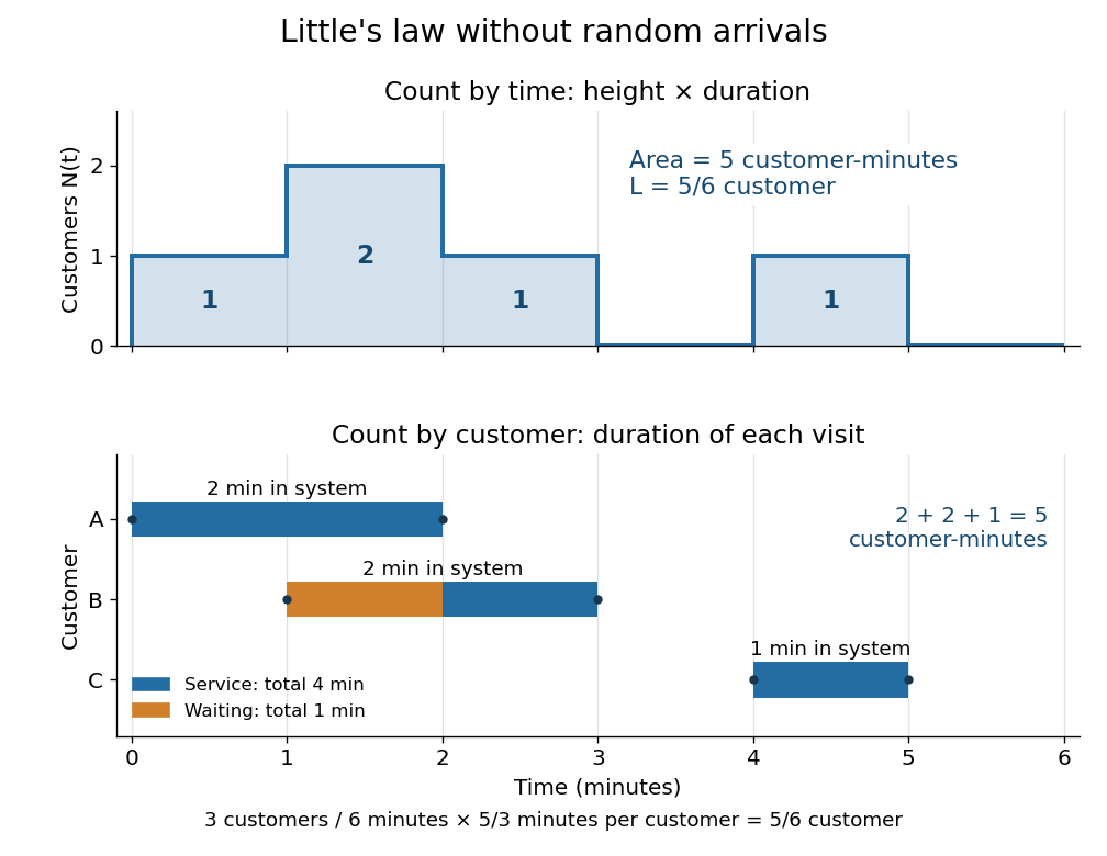
An observation window that cuts visits short requires the overlap terms, rather than full customer sojourn times. Starting empty, let $A(T)$ count admissions before $T$ and write $w_k=d_k-a_k$. ThenFor the example cut at $T=2.5$ minutes, the area is $1+2+0.5=3.5$ customer-minutes, whereas the full durations of the two admitted customers sum to $4$; the remaining half-minute of the second visit is $R(2.5)=0.5$. A precise sufficient sample path condition for the limiting Little's law is $A(T)/T\to {\lambda }_{\mathrm{eff}}\in (0,\infty )$, $A(T{)}^{-1}{\sum }_{a_k<T}{w}_k\to W<\infty$, and $R(T)/T\to 0$. Dividing the identity by $T$ then gives $L={\lambda }_{\mathrm{eff}}W$. Equating admission and departure rates additionally uses $N(T)/T\to 0$, by the balance $N(T)=A(T)-D(T)$ for an initially empty queue, where $D(T)$ counts all departures.