
Two uniform horizontal magnetic fields on either side of a horizontal interface exert no bulk force, but their magnetic pressures differ. For a common-temperature isothermal atmosphere with sound-speed squared and gravity , hydrostatic equilibrium gives and , . Continuity of magnetohydrodynamic total pressure gives the displayed density jump. A stronger field below means denser gas above, supplying a Rayleigh-Taylor instability even though each half-space is hydrostatic.
// Target: continuum-mechanics.bigb
Convective collapse Created 2026-10-14 Updated 2026-11-05
A compressible intensification mechanism for a thin, nearly vertical flux tube in a superadiabatic atmosphere. An unstable downflow drains material and lowers internal gas pressure; approximate lateral balance then permits the tube to contract and its field to strengthen at nearly conserved magnetic flux. It relies on compressibility and thermal evolution, which are absent from a strict Boussinesq approximation. Dynamic photospheric structures need not satisfy thin-tube equilibrium, so this mechanism does not explain every intense field concentration.
Equipartition magnetic field Created 2026-10-14 Updated 2026-11-05
Equating magnetic energy density to kinetic energy density defines this order-of-magnitude field. It marks when a weak-field kinematic treatment of a given flow can fail, not a universal upper bound on concentrated fields. Gas-pressure confinement, compression, partial evacuation and dynamic pressure can allow stronger local fields.
Current-loop torque experiment 2026-10-14
The PHYWE guide Magnetic moment in the magnetic field makes the magnetic dipole moment measurable. A circular test current loop sits between a pair of Helmholtz coils, with separate supplies and meters for the test electric current and field-producing electric current . The test current loop is mounted on a torsion dynamometer. The guide varies , the number of turns, the test electric current, diameter, and the angle between the magnetic dipole moment and magnetic field. Its angular settings are spaced by . The leads hang loosely and are twisted together to suppress extra torque; the instrument zero is checked frequently because moving leads can shift it. Its reported results include approximately linear dependence on each electric current and on winding count, and approximately quadratic dependence on diameter.[ref]
The readout is a balance of torques. According to the manufacturer's Torsion dynamometer 0.01 N operating instructions, a metallic band supplies the restoring torque. First set the indication to zero with the applied force absent and center the lever using the zero knob. Apply the load, then turn the indicating knob until the lever returns to its original zero position. The scale then reads a force equivalent, not a torque directly. The quoted scale division is . For a force applied perpendicular to the calibration lever arm at distance , the conversion is ; a current loop applies a couple, so its torque must be compared with the calibrated restoring torque.[ref]
Torsion dynamometer 0.01 N operating instructions. §§1–4: metallic-band compensation, zero procedure, force indication and scale specification
For a quantitative repeat, independently check that conversion with known forces at a measured perpendicular lever arm, and check the imposed magnetic field at the test current loop. These are proposed calibration checks, not additional measurements reported here. The ideal Helmholtz coil model predictswhere and are the winding count and radius of each field-producing Helmholtz coil, distinct from and of the test current loop. Derive by adding the on-axis magnetic field of a circular current loop at distances from both coils. Independently calibrating and the restoring torque lets a fitted torque amplitude determine as amplitude divided by , to compare with .
Useful additional controls are to reverse only , reverse only , and reverse both: the signed torque should reverse in either single reversal and be unchanged in the double reversal. Record baselines with each electric current separately zero, and subtract a nearby zero reading to reduce torsion balance zero drift. Repeat angular settings in both directions to reveal lead-dependent offsets. These are suggested controls. Limits include finite magnetic field uniformity, uncertainty in effective winding area and angular zero, meter calibration, Joule heating, and residual lead torque. An apparently sinusoidal trace alone does not establish the absolute magnetic dipole moment. No raw laboratory data or new measured values are claimed here.
A nonuniform angular velocity winds an azimuthal magnetic mode into phase . Its radial phase gradient grows as , creating small scales even when its ideal amplitude does not decay. The corresponding leading resistive damping rate is , so a local short-wavelength estimate gives damping factor . Hence magnetic diffusion can become important at time although it is initially small. This is a local phase-mixing estimate, not a globally exact solution in a finite radial domain: boundary forcing, field stretching and spatial variation of must also be retained there.
Localized interchange criterion for a magnetized atmosphere Created 2026-10-14 Updated 2026-11-05
For disturbances constant along the horizontal magnetic field, the minimized energy density is . If its coefficient is nonnegative everywhere, the full energy is nonnegative. If it is strictly negative at a point of a smooth equilibrium, a compactly supported vertical displacement in a neighbouring interval gives negative energy. These interchange motions compress gas and magnetic pressure together.
Isothermal interchange criterion for magnetic buoyancy Created 2026-10-14 Updated 2026-11-05
A horizontal flux tube displaced without bending preserves by magnetic flux freezing. If thermal exchange keeps its temperature equal to its new surroundings, lateral magnetic pressure balance gives . Here , , and primes denote the response to a small vertical displacement from an equilibrium. Its linear buoyancy acceleration is . Thus local interchange is unstable when , equivalently . This fast-thermal-exchange criterion differs from the adiabatic localized interchange criterion for a magnetized atmosphere.
Supermembranes 2026-10-14
The supersymmetric M2-brane worldvolume theory includes embedding bosons and fermions and has kappa symmetry. In eleven dimensions its fermionic embedding coordinate is a thirty-two-component Majorana spinor.
M2-brane supergravity solution 2026-10-14
The transverse harmonic function solves the field equations away from membrane sources. Positive centres contribute in eight dimensions. Its Killing spinors are with one oriented membrane projector, giving sixteen supersymmetries. The three-form's sign and membrane orientation must be chosen together.
Sandwich variance of an M-estimator Created 2026-10-14 Updated 2026-11-05
For an estimating equation with population root , let be nonsingular and . Differentiating the contaminated population equation gives influence function . A consistent sample root with differentiable local expansion satisfies , so the central limit theorem gives the displayed covariance. In the scalar case this is .
If has a finite resolution by finitely generated projective modules, restriction of the semidirect-product group ring gives a direct sum of copies of , indexed by the integers. On its kernel cohomology the cyclic generator shifts those copies, possibly twisting each copy by an automorphism. Invariants are zero because elements have finite support; coinvariants identify with a single copy. The two-column Lyndon–Hochschild–Serre spectral sequence therefore gives the displayed isomorphism of abelian groups. A group with such a finite resolution and cohomological dimension has , so the cyclic extension has dimension .
Assume optically thin photoionization equilibrium and an absorber depth of order its local Jeans length, , where is the local gas fraction. Then . Solving for and substituting in gives the displayed correction. Thus the ionized mass integral weights the neutral-hydrogen column-density distribution by rather than . This model does not apply without modification to optically thick systems or arbitrary unconfined gas.
For a finite open cover of , take continuous nonnegative functions summing to one and positive only in . Such a partition of unity comes from normalizing the distance to a set functions . The Borsuk-Ulam theorem applied to gives equal values at an antipodal pair. The sum condition makes equal too, and some common positive value places both points in one .
Let be the vertices of a regular simplex centered at zero in . The displayed spherical Voronoi cells are a closed cover by sets. If and belonged to the same cell, all their scalar products with the vertices would coincide. Their sum is zero and the vertices span the ambient vector space, so this would force , a contradiction. Thus each cell contains no antipodal pair. Together with the Lusternik-Schnirelmann-Borsuk theorem, this shows is the minimum number of antipodal-free members of a finite closed cover.
For smooth no-slip spheres of radius scale with minimum gap , the lateral gap scale is . Squeeze-film lubrication theory gives pressure and the displayed normal resistance. Bounded forcing therefore gives , so the gap cannot vanish in finite time. The conclusion uses smooth surfaces, no slip and continuum creeping flow; it is not a contact model for rough particles.
For an inner sphere of radius , outer radius , and signed offset along a fixed axis, the leading lubrication pressure generated by offset speed is . Its force on the inner sphere is along that axis. Remove the spatially constant divergent term before taking ; the resistance then tends to . As , it is to leading order.
Axial rotational resistance of eccentric nested spheres Created 2026-10-14 Updated 2026-11-05
For , the crawling speed is . At prescribed , eliminate to obtain . The derivative in vanishes only at , and the dissipation diverges at both endpoints. The displayed optimum still dissipates times the simple Couette flow dissipation of an externally driven flat foot moving at speed across a uniform film of thickness .
LU factorization and solve costs 2026-10-14
For classical dense Gaussian elimination over the real numbers, count each scalar addition, subtraction, multiplication or division as one arithmetic operation. At step , there are elimination multipliers to divide out and remaining entries, each requiring one multiplication and one subtraction. Thus this implementation's unpivoted factorization count isHere uses Big O notation. Partial pivoting adds comparisons and row movement, leaving the leading arithmetic count unchanged. The leading count agrees with the standard dense LU decomposition analysis.[ref]
With unit , forward substitution uses arithmetic operations. Back substitution uses another plus diagonal divisions. Together these cost per right-hand side; applying a stored row permutation moves entries and requires no scalar arithmetic. In Big O notation, Reusing LU factors for multiple right-hand sides therefore costswhereas refactorizing for each of the right-hand sides costs . For and , the leading counts are about versus arithmetic operations, nearly a tenfold saving. These are operation counts, not measured runtimes: memory access and optimized matrix multiplication also affect speed.[ref]
Fundamentals of Numerical Computation by Tobin A. Driscoll and others. §2.5.2, Important note after Definition 2.5.2: flop counts are a rough runtime model; the numerical comparison here is an original calculation
When a fixed matrix is used with several forcing or measurement vectors, compute its Pivoted LU decomposition once. Collect right-hand sides into the columns of , and the corresponding solutions into . ThenEach column undergoes the same row permutation, forward substitution and back substitution. Neither , nor depends on . This is the useful separation between preparing a linear system and applying its solution procedure repeatedly. LAPACK implements it by taking previously computed factors, permuting all right-hand sides, and performing the two triangular solves.[ref]
For the unpivoted factors in Computed three-by-three LU decomposition, takeDirect matrix multiplication checks all three identities , and . The first column reproduces the previous solve; the other two use exactly the same factors. New right-hand sides can also arrive one at a time. If changes, these stored factors generally need to be recomputed.
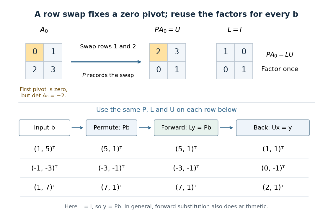
One row permutation fixes a zero pivot element; each new right-hand side reuses the same LU decomposition and two triangular solves
. Details. 
There are unlisted articles, also show them or only show them.