
Aperture dependence of mass-to-light ratio Created 2026-10-14 Updated 2026-11-05
A dynamical mass-to-light ratio must specify its aperture and whether the mass includes dark matter. A growing dark halo can increase outside the bright stellar body even when the stellar ratio is constant. Comparing a tidal-radius satellite mass with a large-aperture host mass is different from comparing both within their half-light radii. From and , the inferred ratio scales as , so equal ratios additionally require homologous radius scaling.
Bounded-coefficient asset deflator Created 2026-10-14 Updated 2026-11-05
Work in discounted units with a unit bank account and a square invertible volatility matrix. For asset dynamics , let and . The Itô product rule cancels the drift of each , leaving the displayed stochastic integral. When is bounded and , is bounded and the Novikov condition makes a true martingale on every finite horizon. If is also bounded, each satisfies the Novikov condition as a stochastic exponential with bounded integrand , so it too is a true martingale.
Equality in Markov's inequality Created 2026-10-14 Updated 2026-10-25
For a finite-expected value nonnegative random variable and , equality in the uncapped Markov's inequality holds exactly when takes only and almost surely. Indeed the nonnegative difference has zero expected value exactly when it vanishes almost surely. Giving probability yields and . This shows the bound cannot generally be reduced using only the nonnegative random variable's expected value.
Markov semigroup 2026-10-14
The transition operators of a time-homogeneous Markov process satisfy by the Markov property. They preserve constants and positivity. When the generator and function domain permit differentiation, is the Kolmogorov backward equation. Transition semigroup of a continuous-time Markov chain is the discrete-state special case.
If a real degree-at-most- polynomial has absolute value at most one at every extremum of the Chebyshev polynomial , its th derivative on is bounded by , for . This strengthens the Markov inequality for polynomial derivatives by replacing a bound on the whole interval with these finitely many samples. The node set is rigid, as quantified by uniqueness of Chebyshev derivative-norming nodes.
Coupling from the past 2026-10-14
Coupling from the past uses a fixed two-sided sequence of random update maps for a finite Markov chain. Increase a backward horizon until the composition from that horizon to time zero sends every starting state to the same state. Retain the maps at previously exposed times. The resulting common image is an exact stationary sample. If a length- block has positive probability of mapping every state to one state, independent disjoint blocks imply failure to coalesce by horizon has probability at most . For a deterministic horizon, a stationary initial state yields a stationary final state, and agrees with the algorithm's output on coalescence. Letting the deterministic horizon tend to infinity proves the output has the stationary law without conditioning on a random stopping horizon.
MCMC trace diagnosis and proposal tuning Created 2026-10-14 Updated 2026-10-20
A trace of a Markov chain Monte Carlo parameter helps distinguish slow movement, long rejection plateaus, and movement between separated regions. Very small random-walk proposals give high acceptance but slow diffusion; very large proposals produce low acceptance and repeated states. Record acceptance rates alongside trace plots and effective sample size of a Markov chain before deciding which scale to change. Correlated posterior directions often benefit from block proposals with a covariance fitted during a preliminary tuning run. A trace alone cannot prove convergence or identify the unique cause of poor movement; dispersed chains and stationary summaries provide additional evidence. Freeze tuning before the main sampling phase, or use adaptation satisfying an appropriate ergodicity theorem.
Stochastic matrix 2026-10-14
A row-stochastic matrix has nonnegative entries and each row sums to one. For a time-homogeneous Discrete-time Markov chain, its transition matrix has entriesIf a state has zero probability at time , this row is specified by the model's Markov kernel, rather than recovered by conditioning on that zero-probability event. Rows index departure states and columns arrival states. Writing the current probability distribution as a row vector givesThe row-sum condition ensures that matrix multiplication preserves total probability. Under a column convention the evolution uses the transpose; the convention must accompany the formula.
For the sunny/rainy transition matrix, direct matrix multiplication givesIn particular, . The two terms sum the disjoint paths and . Requiring both subsequent days to be sunny has probability ; requiring only the second day to be sunny permits the extra path through rain.
Generally is the -step transition probability. The identity is the discrete-time Chapman-Kolmogorov equation: sum over the intermediate state. This makes matrix powers useful for forecasting many steps without enumerating every path individually.
Nonnegative superharmonic function for a Markov chain Created 2026-10-14 Updated 2026-11-05
For a transition matrix , a finite-valued function on its state space is nonnegative superharmonic when . Thus and its expected value cannot increase after one step. Replacing transitions on a target set by identity rows preserves . Iterating this inequality gives , a useful bound for hitting probabilities without a separate optional-stopping theorem.
Discrete-time Markov chain martingale characterization Created 2026-10-14 Updated 2026-11-05
An adapted process on a finite or countable state space has the Markov chain transition matrix exactly when the displayed process is a martingale for every bounded test function . The forward implication follows by taking the conditional expectation of its increment. Conversely, the Martingale property gives ; testing individual-state indicators recovers the entire conditional transition law. Stopping these martingales turns equations and into hitting probabilities and expected hitting times.
Discrete-time Markov chain 2026-10-14
A time-homogeneous Discrete-time Markov chain is a sequence of random variables indexed by nonnegative integers, with the displayed conditional probabilities. Here is its natural filtration and is a row-stochastic transition matrix. The Markov property removes dependence on earlier observations once is specified; the time-homogeneous Markov property makes independent of .
Consider states (sunny) and (rainy), with the constructed transition matrixRows give today's state and columns tomorrow's, in order . These numbers define an illustrative model, with one step interpreted as one day; they are not estimates of real weather. Let . The law of total probability gives the recurrence relationSubtracting makes the deviation multiply by at each step. ThusStarting sunny gives , , and ; starting rainy gives and . The two predictions approach the same stationary distribution while retaining a shrinking trace of the initial probability distribution.
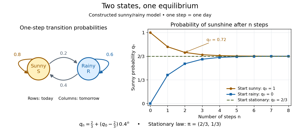
Constructed sunny/rainy transitions and the exact sunny probabilities from three initial distributions.
Details. 
An expected hitting time answers a different question. Starting sunny, let . Every day before the first rain remains sunny, soThis geometric distribution has finite expected value. A first-step calculation gives , with , hence days. The same result follows from the geometric series . This is a mean waiting time, not a prediction that rain first occurs exactly five days later.
A probability row vector is a stationary distribution when . The Markov chain is reversible in that law when detailed balance holds: . Multiplying those equations along a finite path gives equal forward and reversed stationary path probabilities.
Last-excursion direction law at a transient junction Created 2026-10-14 Updated 2026-11-05
At a junction, let be the Probability that one excursion leaves through branch and never returns. If , repeated returns restart the same probabilities by the Strong Markov property. Thus the Probability of returns is , and eventual escape through is . When the branches have outward random-walk drift, the final infinite excursion tends to the corresponding end almost surely.
Reflected chain with geometric downward jumps Created 2026-10-14 Updated 2026-11-05
Fix and put . For independent geometric random variables with for , the Reflected chain with geometric downward jumps obeys . Its transition probabilities are for and .
The Probability of hitting zero from is one when and when . The first-step boundary equation at is essential for the extra exponent. Before reflection the mean increment is : downward drift corresponds to .
The chain is positive recurrent for , with Stationary distribution for . The ratio ensures these weights sum to one. It is null recurrent at and transient for . The parameter restriction matters: does not define the displayed geometric distribution, and produces deterministic upward motion rather than an irreducible chain.
Jump chain of a discrete-time Markov chain 2026-10-14
For , observe a discrete-time Markov chain only when its state changes. The probability that its next different state is is . Its holding times are finite geometric waiting times. This construction deletes self-transitions and differs from the existing continuous-time jump-chain concept.
Take states for , with deterministic and transitions with probability , with probability , with probability , and with probability . The Markov chain is transient for , null recurrent for , and positive recurrent for . To see the Markov chain recurrence threshold, eliminate the primed-state hitting probabilities to obtain , with characteristic roots and . Boundedness forces return with probability one when the second root is at least one. When it is below one, the minimal nonnegative solution gives return probability from . In the positive recurrent case, put and . The stationary distribution is , and . It follows from balance across each level cut and sums to one; at criticality the invariant weights cannot be normalized.
Harmonic function for a Markov chain Created 2026-10-14 Updated 2026-10-20
A harmonic function assigns a value to each state of a Markov chain such that one transition leaves its expected value unchanged. This turns a question about many possible future sample paths, such as which endpoint is reached first, into a local averaging rule. For a transition matrix , a real-valued function is harmonic at state whenHere means expected value conditional on starting at ; on a countable state space the sum must be absolutely convergent. If this holds at every state, write . At an absorbing state the equation is automatic, so prescribed boundary conditions supply information that the averaging rule cannot.
For a finite Markov chain, choose a boundary set that can be reached from every state, and assign boundary values . If is its first hitting time, the harmonic extension isChoosing to be the indicator function of one target within gives a hitting probability. This is a discrete Dirichlet problem: enforce the averaging rule outside and fix the values on . See Hao Wu's MIT lecture 8, harmonic extension, slide 5. The construction extends the mean-value idea of a harmonic function; for a random walk on a graph it is a discrete harmonic function.
Capital market line 2026-10-14
In mean-variance optimization with unrestricted borrowing/lending, the upper efficient ray through the risk-free point has slope . If , it touches the risky efficient frontier at the positive-premium normalized market portfolio. The Sharpe ratio there equals the slope. If this normalization is negative, the normalized tangency portfolio instead has negative excess return; the upper ray uses a short position in that portfolio and is not tangent to the upper risky branch.
Sign of the normalized tangency portfolio 2026-10-14
Assume a positive definite covariance matrix and nonzero excess-mean vector . The Cauchy-Schwarz inequality gives , with the positive-premium efficient direction , . If , its normalized risky portfolio has Sharpe ratio . Thus negative normalization reverses the efficient orientation. If , the efficient risky direction is self-funded and cannot be normalized to a unit risky budget.
Capture-recapture model 2026-10-14
A capture-recapture model is a statistical model for repeated observations of identifiable individuals, including those missed on some occasions. A closed-population capture-recapture model estimates a fixed population cardinality; models allowing individuals to enter or leave can instead describe survival and recruitment. The sampling assumptions determine which likelihood function is appropriate.
For the two-sample closed-population capture-recapture model, condition on the sample sizes and . If the second sample selects distinct individuals from by simple random sampling, then the overlap has the hypergeometric distribution:Here is an integer and the probability mass function is zero outside these bounds. The binomial coefficients count choices of marked and unmarked individuals, divided by all equally likely size- subsets. The hypergeometric distribution has expected valueEquating the observed overlap with this expected value gives the Lincoln-Petersen estimator. The underlying sampling without replacement, probability mass function, and expected value are developed in Raymond P. Guiteras, MIT 14.30 hypergeometric distribution handout, §§1–4 and 8.
For the toy counts , , and , hold the observations fixed and vary the unknown integer . The likelihood function isValues below forty cannot contain the observed set union. Exact comparison of consecutive likelihoods gives two tied maximum-likelihood estimates, and . The Lincoln-Petersen estimator returns ; the Chapman estimator returns and is a different rule for estimation.
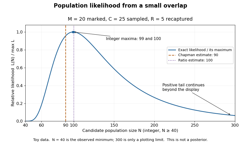
Relative likelihood for the toy overlap: integer maxima at 99 and 100, ratio estimate 100, and Chapman estimate 90
. Details. 
The vertical scale is . This relative likelihood compares how well candidate statistical parameters explain the same observations; it is not a posterior probability. The displayed range is only a plotting window. The likelihood function remains positive for every integer and tends to zero as increases, so the curve has a continuing right tail. The data do not justify truncating statistical inference at three hundred. The conditional hypergeometric distribution formulation also appears in Louis-Paul Rivest and Mamadou Yauck, Small Sample Estimators for Two-way Capture Recapture Experiments, §3, equation (5).
Zero recaptures require care. With and positive , the Lincoln-Petersen estimator has no finite ratio, but the capture-recapture model still gives a valid likelihood function:This likelihood function increases toward one as grows, so there is no finite maximum-likelihood estimate. For the same sample sizes twenty and twenty-five with zero overlap, forty-five distinct individuals would be observed. Lack of overlap supplies a lower bound but very weak information about large population cardinalities.
In more elaborate capture-recapture models, a first-recapture array counts individuals released at occasion and next observed at . A probability of survival and a probability of detection contribute a no-observation continuation factor . The resulting likelihood function depends on both survival and detection; these probabilities need not be separately identifiable at the last observation interval. Missing-count EM for capture-recapture describes one way to fit such a model, and identifiability remains a separate issue from computing an estimator output.
Puppe sequence 2026-10-14
Successive mapping cones of a based map give this sequence up to homotopy. Applying based maps into a space gives an exact sequence of pointed sets in the opposite direction. The exactness statement at says that a map whose restriction to is null-homotopic extends over using the chosen null-homotopy.
There are unlisted articles, also show them or only show them.