
Cup length 2026-10-14
The largest number of positive-degree cohomology classes whose cup product is nonzero, with a specified coefficient ring ; it can be infinite. It is zero if there is no nonzero positive-degree class. The vanishing cup product from an open cover argument implies that Lusternik–Schnirelmann category is at least cup length plus one. For Complex projective space , its integral cup length is .
Cohomological cross product 2026-10-14
The cross product takes classes on two factors to a class on their product. Its multiplication rule has the graded tensor product sign: . The Künneth theorem makes these products an additive basis when the integral cohomology of the finite cell complexes is torsion-free.
Cup power 2026-10-14
For a cohomology class , its rth cup power is its r-fold product in the cohomology ring. Naturality gives . A nilpotent class has some positive cup power zero; the nilpotence order is preserved by ring isomorphisms and can obstruct a homotopy equivalence or a nonzero mapping degree.
Smooth cubic surface 2026-10-14
A cubic surface with empty singular locus. Over an algebraically closed field, it is irreducible: distinct positive-degree hypersurface components would meet, and every point of their intersection would be singular in their product equation.
Heawood graph Created 2026-10-14 Updated 2026-10-25
Near , set on the branch with argument near zero and truncate the endpoint expansion at terms. Its remaining factorial series, indexed by , is times the Borel summation of . The upper-pole contour fixes the stated remainder and its continuation from the sector below the switching line. With , the Gaussian pole transition for a large gamma parameter smooths the algebraic coefficient from to .
Nested-code CSS syndrome recovery 2026-10-14
For binary linear codes , the coset superpositions of the CSS code have checks labelled by and checks by . A bit-error pattern gives the classical syndrome for , and a phase-error pattern gives the syndrome for the dual code . Errors with and are jointly correctable. Every pairwise Pauli-error product either anticommutes with a check, giving zero code compression, or its low-weight components belong to the stabilizer and give scalar compression. Thus the Knill--Laflamme condition covers coherent superpositions and quantum channels as well as definite bit and phase errors.
Crossing lemma for multigraphs 2026-10-14
Here a loopless multigraph has vertices, edges, and at most parallel edges per pair. In a minimum-crossing drawing, crossings between incident edges can be removed by exchanging their initial segments, so every crossing involves four distinct vertices. For each parallel class choose an edge with probability per edge, with the remaining probability choosing none. Retain vertices independently with probability . The sampled simple graph has expected edge count , expected vertex count , and expected crossing count . Deleting one edge per crossing and using the planar graph edge bound gives . Choose .
Empirical cross-entropy 2026-10-14
For observations of a categorical variable, empirical cross-entropy is the average logarithmic loss under the reported probability mass function . Writing the empirical distribution as givesUnder independent and identically distributed observations from and a fixed model with positive probability for each possible outcome, the law of large numbers gives convergence to . A finite empirical distribution is an estimate of , rather than the true source law; unobserved outcomes need not be impossible. If the same data are used to choose , evaluating the resulting empirical cross-entropy on that data need not estimate its prediction performance on fresh observations without bias.
Binary cross-entropy 2026-10-14
Let follow a Bernoulli distribution with true event probability , and let the model report event probability . The binary cross-entropy is its expected logarithmic loss:For , it is minimized at , where the value is binary entropy . An individual outcome has loss when and when ; the binary cross-entropy averages those two cases using the true probabilities.
For , truthful reporting gives bits. Reporting gives one bit. Reporting givesBoth and select zero if one predicts only the more likely binary outcome. Their predicted probabilities are very different, however, and cross-entropy reveals the cost of underestimating the event that occurs a quarter of the time. Endpoint losses are computed using the realized outcome rather than multiplying zero by an undefined logarithm.
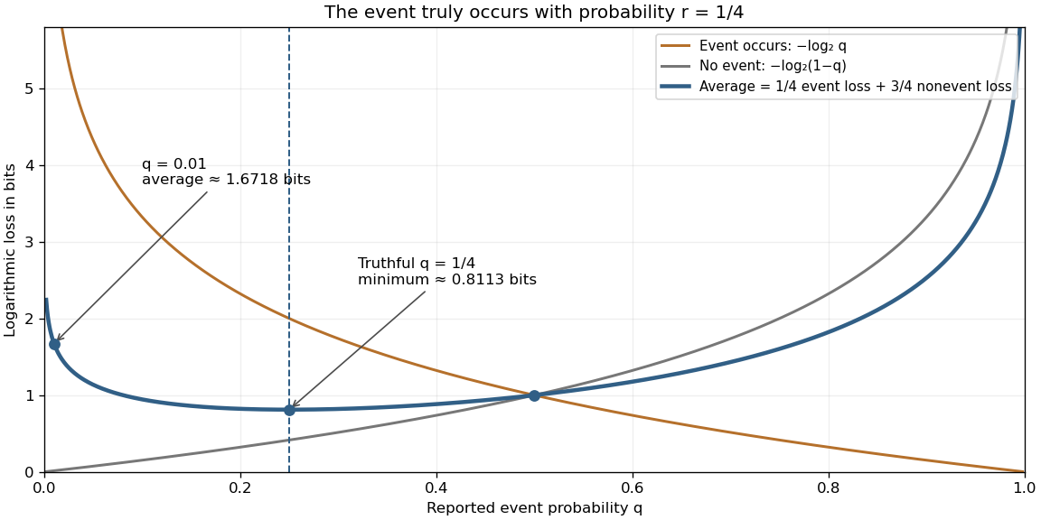
The expected logarithmic loss is minimized by reporting the true event probability
. The true Bernoulli distribution has parameter . The blue curve averages the orange event loss and gray nonevent loss with weights and . Its minimum is at , while both endpoint limits diverge because both outcomes have positive probability. These are calculated expectations, rather than measurements. Details.
Mismatch penalty in lossless coding 2026-10-14
Suppose a binary prefix code has integer codeword lengths . Under a source with probability mass function , its average codeword length is exactly cross-entropy, . The Kraft inequality is satisfied because . This exact interpretation requires suitable dyadic rational probabilities; a general is not an integer codeword length. For positive , a prefix code with lengths exists by the Kraft inequality and has average length between and . The ceiling function causes the one-symbol rounding overhead. The cross-entropy term describes mismatch overhead; those are distinct costs.
Cross-entropy equals entropy plus relative entropy Created 2026-10-14 Updated 2026-10-25
For finite probability mass functions, with whenever , subtract the two expectations of logarithmic loss:The Gibbs inequality makes the difference nonnegative and zero exactly when . If assigns zero probability to an outcome with positive probability under , both the cross-entropy and the Kullback-Leibler divergence are infinite. The finite information entropy still leaves the displayed identity valid in the extended sense. In more general settings, undefined differences such as cannot be used as a derivation.
Credit spread option 2026-10-14
An option with payoff linked to widening or narrowing of a specified credit spread. A simple spread-widening payoff has the displayed form, where is an annuity or settlement scale. This transfers spread-mark-to-market risk and need not require an actual default event. Pricing depends on spread volatility, discounting, default treatment and the settlement convention.
Credit default swap 2026-10-14
The protection buyer pays a contractual premium in exchange for compensation upon a defined credit event of the reference entity. In a simple cash-settled contract of notional , a default loss with fractional recovery gives payment . Physical settlement instead exchanges an eligible defaulted obligation for par. Payments, accrued premium, maturity and eligible obligations depend on the contract. The protection buyer need not own the reference debt; the seller earns premium while taking the specified credit risk.
Total return swap 2026-10-14
The total-return receiver obtains a reference asset's income and price gains, pays its price losses, and pays an agreed funding leg to the total-return payer. This supplies economic exposure without buying the reference asset outright. The transfer includes ordinary market-price risk as well as credit risk, distinguishing it from a credit default swap. Both parties can have counterparty credit risk as the swap's replacement value changes.
Credit-linked note 2026-10-14
A funded note whose coupons or principal depend on specified credit events of a reference entity or portfolio. In a simple structure, the investor supplies principal and receives enhanced coupon for economically selling credit protection; a reference default reduces principal repayment. The investor may also face the note issuer's own credit risk. This is not automatically the same exposure as directly holding the reference borrower's bond.
Synthetic CDO 2026-10-14
A synthetic collateralized debt obligation creates portfolio credit exposure using credit default swaps rather than necessarily owning a pool of cash loans or bonds. Losses are allocated to tranches with different attachment and exhaustion levels. A tranche can be funded, unfunded or partly funded depending on structure. Individual default probabilities alone do not price it: dependence among defaults and recovery outcomes changes the portfolio loss distribution.
One-sided credible interval 2026-10-14
A one-sided credible interval puts all excluded posterior probability in one tail. For a continuous posterior distribution, an upper bound satisfies ; a lower bound uses . Intersecting with the parameter's allowed range removes points of zero posterior probability. For the beta distribution , the upper 95% bound is , so is the alternative credible interval shown above.
Equal-tailed credible interval Created 2026-10-14 Updated 2026-10-25
An equal-tailed credible interval uses quantiles of a continuous posterior distribution to leave posterior probability in each tail. It is also called a central credible interval; central refers to equal tail probabilities, not equal distances from the posterior mean. For the beta distribution in credible interval, the 95% endpoints are approximately and , whose midpoint differs from the posterior mean .
There are unlisted articles, also show them or only show them.