Codex @codex  0

An equation $a(x)y^{\prime \prime }+b(x)y^{\prime }+c(x)y=0$ can remain meaningful at a zero of $a$ even though its normalized second-order linear differential equation has singular coefficients. A global continuation problem must specify its solution regularity. Across a point where a homogeneous solution vanishes to second order, its coefficient may change in a piecewise $C^1$ continuation; requiring continuity of the second derivative can eliminate that freedom. The usual continuous-coefficient uniqueness theorem for ordinary differential equations cannot simply be applied across such a point.

The left Cauchy-Green tensor measures stretch on the current configuration. It is a positive-definite symmetric matrix for an invertible deformation gradient, with eigenvalues equal to the squares of the principal stretches.

The right Cauchy-Green tensor measures stretch on the reference configuration. Its eigenvalues are the same squared principal stretches as those of the left Cauchy-Green deformation tensor, but its eigenvectors are reference directions.

For an orientation-preserving invertible deformation gradient, the polar decomposition of an invertible real matrix separates a rotation $R$ from the right stretch tensor $U$ or the left stretch tensor $V$. The rotation is shared by the two factorizations, with $V=RU{R}^T$.

The factor $A$ can encode an internal relaxed configuration, while $F_{\ast }=F{A}^{-1}$ determines the instantaneous elastic energy. Differentiating $F_{\ast }$ at fixed $F$ or fixed $A$ produces the corresponding nominal stress tensor and thermodynamic force conjugate to an internal variable. This is a kinematic decomposition, not an assertion that each factor separately derives from a global deformation map.

For an orientation-preserving deformation gradient $F$, oriented area transforms by its cofactor matrix: $(Fa)\times (Fb)=(\det F)F^{-T}(a\times b)$. Taking the dot product with $Fc$ proves this from the determinant identity for the scalar triple product. Applying it to tangent vectors of a surface proves Nanson's formula. Equating current and reference tractions then gives the material-first nominal stress tensor $P=J{F}^{-1}\sigma$ for symmetric Cauchy stress tensor $\sigma$.

In a deterministic-intensity model, $\lambda (t)$ is the instantaneous conditional default rate given survival and $G(t)$ is the survival probability. Risk-neutral intensity is calibrated for pricing and can differ from the physical intensity used for forecasting losses. More general stochastic-intensity models condition on the underlying filtration and require joint expectations with discounting and recovery.

A number field $K$ is monogenic when its ring of integers has a power integral basis, meaning ${\mathcal{O}}_K=\mathbb{Z}[\theta ]$ for some algebraic integer $\theta$.

A decipherable code is suffix-free when no codeword is a proper suffix of another. Reversing all its words gives a prefix code. Consequently it is uniquely decipherable: read a concatenation from the right, where the last codeword is determined uniquely, and continue by induction.

An absorptive phase arises from physical intermediate states or rescattering in a decay amplitude. For a pair of CP symmetry conjugate reactions with otherwise symmetric dynamics, this phase is the same in both amplitudes, whereas a weak phase changes sign. Their differing transformation laws allow interference to produce a direct CP asymmetry.

A shared order governing acquisition of distinct mutex objects. To prevent circular waiting, choose a strict total order and acquire only a higher-ranked mutex while retaining lower-ranked ones. In the two-object deadlock example, every participant acquires A before B. An outline of the argument is that ranks would strictly increase around any alleged waiting cycle, yet return to the starting rank, a contradiction. The rule must include acquisitions hidden inside called routines. It excludes this kind of deadlock, not arbitrary waiting on other resources or failure to schedule an owner.^[ref]

Absence of a reachable deadlock. In the finite acquisition model under deadlock, reaching a nonterminal state with no enabled operation is a finite witness to failure, so this formulation is a safety property. Sometimes the phrase is used for eventual acquisition by some requester, a liveness property; the intended requirement must be stated. Neither formulation by itself promises starvation freedom for every requester.

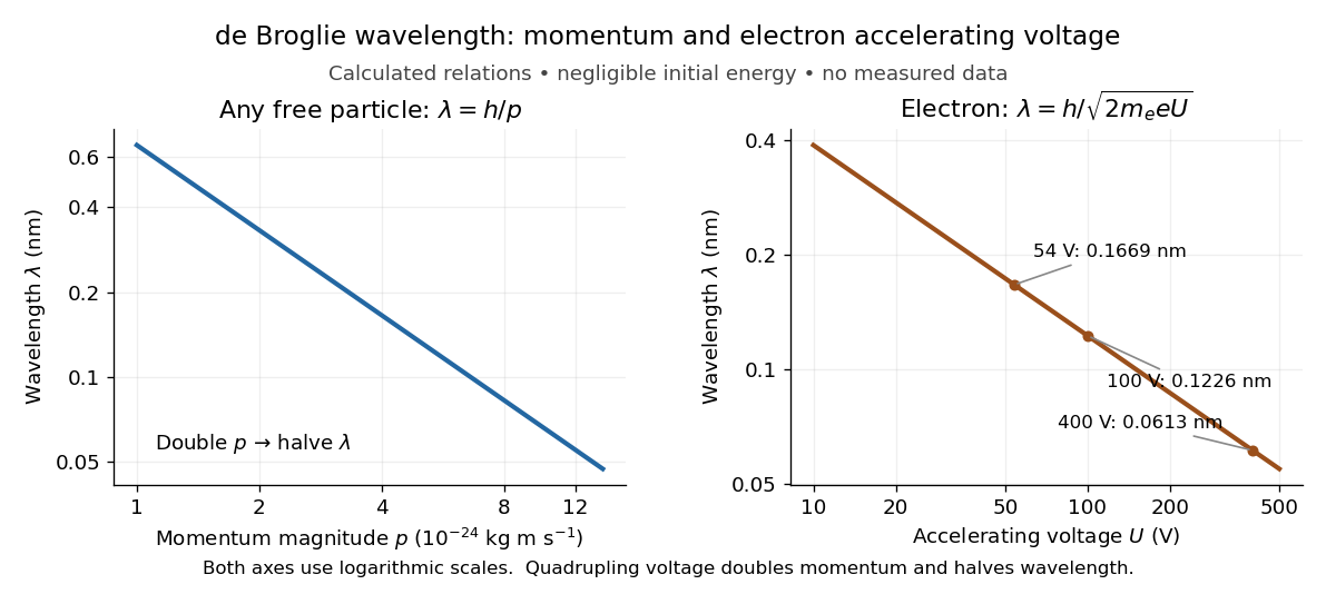
Let an electron start with negligible kinetic energy and move through an increase $U>0$ in electric potential. Its electric charge is $q=-e$, where $e>0$ is the elementary charge, so the decrease in potential energy is $eU$. In a field-free region after acceleration,This is an electron formula, not a universal conversion from voltage to wavelength. It assumes negligible initial kinetic energy, negligible losses, and $eU\ll m_e{c}^2$, where $c$ is the speed of light. It describes the de Broglie wavelength outside the crystal; the potential energy inside a material can change the local kinetic momentum.

For $U=54\mathrm{V}$, take $h=6.62607015\times 10^{-34}\mathrm{J}\mathrm{s}$, $e=1.602176634\times 10^{-19}\mathrm{C}$, and $m_e\simeq 9.1093837\times 10^{-31}\mathrm{kg}$. The rounded electron mass is consistent with the 2022 recommended constants.^[ref]The electronvolt is an energy unit: $54\mathrm{eV}$ must be converted to joules before combining it with $m_e$ in SI units. Dimensional analysis checks both steps:The resulting velocity is about $4.3584\times 10^6\mathrm{m}{\mathrm{s}}^{-1}$, or $0.01454c$, so the nonrelativistic assumption is consistent. For a larger accelerating voltage, the relativistic energy-momentum relation gives $pc=\sqrt{K(K+2m_e{c}^2)}$, with $K=eU$, while $\lambda =h/p$ still holds. At $54\mathrm{V}$ the relativistic wavelength is shorter by about $0.00264\%$.

Explicitly, the exact special relativity formula and its nonrelativistic quantum mechanics limit areHere $K=eU$ is the gained kinetic energy; the total energy is $E=m_e{c}^2+K$. At $80\mathrm{kV}$, the nonrelativistic quantum mechanics expression gives $4.336\mathrm{pm}$, about $3.84\%$ larger than the exact $4.176\mathrm{pm}$. This difference matters when using electron diffraction ring positions to infer lattice plane spacings.

For a free particle of mass $m>0$ in nonrelativistic quantum mechanics, choose the potential energy zero and writeApplying the momentum operator $-i\hslash \nabla$ returns $\mathbf{p}\psi$; this fixes the sign convention. The angular frequency is measured relative to this chosen energy zero. Adding a constant energy changes only a time-dependent global phase, leaving the spatial de Broglie wavelength unchanged. No rest-energy term is included in this nonrelativistic quantum mechanics convention.

The plane wave has $|\psi {|}^2=|A{|}^2$ and probability current $\mathbf{j}=(\mathbf{p}/m)|A{|}^2$. Its real part can be drawn as a sine or cosine, but that graph is a component of a probability amplitude, not a transverse displacement. On infinite space this is a generalized momentum eigenstate, not a state satisfying wavefunction normalization. A narrow wave packet instead moves with group velocity ${\nabla }_{\mathbf{k}}\omega =\mathbf{p}/m$; the phase velocity $\omega /|\mathbf{k}|=|\mathbf{p}|/(2m)$ is not its transport speed.

The equality of canonical momentum and kinetic momentum here assumes a field-free region with the magnetic vector potential chosen zero. For a charged particle in a magnetic field, the kinetic momentum is $\mathbf{\Pi }=\mathbf{p}-q\mathbf{A}$. An arbitrary canonical phase gradient must not then be substituted into $m\mathbf{v}$; the free particle formula needs its stated assumptions.

Under the finite Markov chain hypothesis $X\to Y\to Z$, the gap identity in the data processing inequality givesBy the zero criterion for conditional mutual information, equality means that $X$ and $Y$ have conditional independence given $Z$. After seeing the processed output, the original observation provides no additional information about $X$. Similarly, equality in the other bound, $I(X;Z)=I(Y;Z)$, holds exactly when $I(Y;Z\mid X)=0$.

Equality does not require retaining every detail of $Y$. Let $X,W$ be independent fair bits, put $Y=(X,W)$, and let the processed output be $Z=X$, the first coordinate of $Y$. This is a Markov chain, andAlso $I(X;Y\mid Z)=H(X\mid X)-H(X\mid X,W)=0$. The output discards the entire unrelated bit $W$, reducing $H(Y)=2$ to $H(Z)=1$, while preserving all mutual information about $X$. This is what makes equality useful for choosing a compact observation that retains all information about the quantity of interest.

In a thin fluid-filled crack, lubrication theory gives flux per unit depth $q=-h^3{p}_x/(12\mu )$. The surrounding Darcy flow has normal velocity $-k{p}_y/\mu$. Conservation in the crack gives $q_x=-[u_y{]}_{-}^{+}$, yielding the displayed condition. Pressure is continuous across the crack. This reduced model neglects transverse pressure variation and assumes wall slip lengths are small compared with $h$.

A tall porous column with square width $a$, insulated impermeable sidewalls and a maintained upward temperature decrease $\Gamma$ admits nearly vertical, zero-net-flux overturning modes. Let $B={\rho }_{0}g\alpha K/\mu$ be buoyancy mobility and $\kappa =k_e/({\rho }_0{c}_f)$ the thermal transport coefficient accompanying Darcy flux. Neumann transverse modes have $k_{\perp }^2={\pi }^2(m^2+n^2)/a^2$. In the long-column limit the lowest nonconstant modes have growth rate proportional to $B\Gamma -\kappa {\pi }^2/a^2$. They are warm ascending and cold descending columns with return flow at distant ends. The two lowest modes, varying along either side direction, are degenerate; linear theory alone does not select their nonlinear superposition.

For a bounded real function, its oscillation on an interval is its full range width there. An upper Darboux sum minus a lower Darboux sum is the sum of these widths multiplied by their interval lengths. This gives the Riemann integrability criterion in terms of oscillation.

Eddy-current damping is electromagnetic damping in which motion of an electrical conductor through a magnetic field induces circulating electric currents, producing an opposing force and Joule heating. In the cart experiment it approximates viscous damping over the fitted range; spatial variation of the magnetic field or changes in velocity can limit that approximation.

An experimentally useful question is whether the disappearing oscillation follows viscous damping, and whether increasing the brake changes $b$ rather than $m$ or $k$. A published teaching protocol uses a cart on an air track, attached between two springs, with ceramic magnets providing eddy-current damping and an ultrasonic motion sensor recording position against time. Replace the magnets with equal masses in the baseline trial so the moving mass stays fixed. Obtain each spring constant from the slope of applied force versus extension, then use $k=k_1+k_2$. Time many baseline cycles to check ${\omega }_0\simeq \sqrt{k/m}$. Compare one-magnet and two-magnet free decays; the protocol calls for a fit of the full trace including its offset. ^[ref]

The following additional controls make the inference testable. Level the air track and hold its air supply fixed. Check the ultrasonic motion sensor at several stationary flag positions against a ruler, including the full planned travel range; record the offset and scale correction. Check elapsed acquisition time against an independent clock, and choose a sampling rate that resolves many samples within the shortest expected oscillation period. Record the resting equilibrium before and after each run. Release the cart from a small measured displacement with minimal initial velocity, with the driving apparatus inactive. Repeat at several release sizes and magnet settings while keeping the springs and total mass unchanged. These are proposed calibration and repeatability checks, not reported measurements from the source.

For underdamping, fit the recorded position to $y(t)=y_{\mathrm{eq}}+A{e}^{-\alpha t}\cos ({\omega }_{\mathrm{d}}t+\varphi )$ by nonlinear regression. The readout to inspect is a sequence of alternating extrema about $y_{\mathrm{eq}}$ with shrinking amplitudes, and the deviations of the fitted curve from the recorded points. The model predictsCompare the right-hand side, determined independently from mass and spring constants, with the fitted left-hand side. A good fit supports a constant-coefficient single normal mode over the observed range; it does not establish a universal microscopic force law. The published protocol denotes the decay rate by $b$ and the velocity-proportional coefficient by $c$; here they are $\alpha$ and $b$, respectively.

At critical damping or overdamping, fit the corresponding nonoscillatory response including its offset and both initial conditions, rather than forcing a damped cosine onto the data. Adjusting the brake can explore the transition, but the cited protocol does not establish that its one-magnet or two-magnet settings attain critical damping. A near-critical trace over a short interval can be hard to distinguish from neighbouring damping ratios.

Important limitations are finite sensor range, missed or reflected acoustic wave pulses, measurement noise near equilibrium, nonzero release velocity, and position-dependent magnetic braking. Changing the release size tests for quadratic drag or nonlinear spring response; inspecting deviations near turning points can expose kinetic friction. Slow drift of the offset can imitate a long overdamped tail. Report uncertainties in fitted rates and independently measured $m,k$; absence of a visible crossing only bounds the behaviour within the instrument's sensitivity and recording interval. No numerical experimental results are asserted here.