
Coalgebra Created 2026-10-06 Updated 2026-10-20
Coarse-grid correction Created 2026-10-06 Updated 2026-10-14
A coarse-grid correction improves a fine-grid approximation by solving a smaller equation for the part of its approximation error representable on a coarse mesh. Use the signed convention and the linear-system residual . A prolongation linear map interpolates coarse corrections into fine-grid corrections, and a restriction linear map transfers the linear-system residual. Solve exactly or approximately and update . The plus sign follows from defining the approximation error as exact minus approximate. It is the correction equation's right-hand side , rather than merely restricted solution values, that determines the update.
For the multigrid method model , take , so and the coarse nodes coincide with every second fine node. Use linear interpolation with zero boundary corrections :Use full-weighting restriction for the interior linear-system residual:Here is the matrix transpose in ordinary unweighted coordinates. With these specific transfers, the Galerkin coarse-grid operator isThus it equals the rediscretized Poisson equation operator on this constant-coefficient one-dimensional mesh. The equality is special to the stated model and transfers. In particular, dropping from the fine matrix while using on the coarse mesh changes the correction unless the right-hand sides and transfers are rescaled consistently.
Take seven interior points, , three coarse unknowns, and the deliberately constructed approximation errorFor example, choose , so and . Direct matrix multiplication givesThe exact coarse solve returns , so adding removes the entire chosen approximation error. A broad triangular error can have a sharply localized linear-system residual: the latter measures discrete curvature, not error height. This is why the two should not be confused. A smooth sine mode instead has linear-system residual , so interpreting its magnitude also requires the eigenvalue and the equation's scaling.
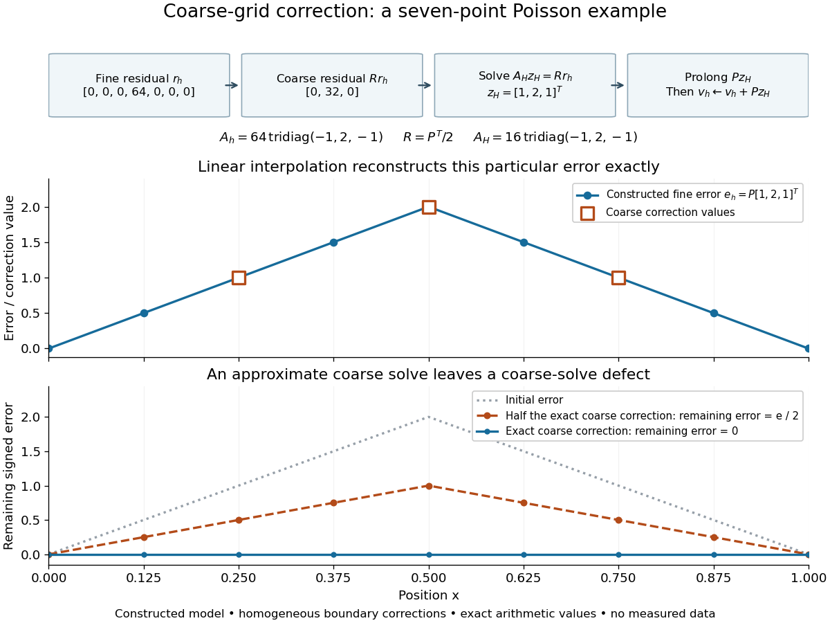
Constructed seven-point Poisson example: residual restriction, coarse solve, interpolation, and the error remaining after exact or partial correction
. Details. 
The algebra explains the exact cancellation beyond this example. Assume has linearly independent columns and choose an invertible Galerkin coarse-grid operator . With an exact coarse solve, the iteration matrix for the remaining approximation error isThe short proof is to substitute . Thus every vector in the column space of is eliminated, and the corrected linear-system residual restricts to zero. These are exact projection identities, not a statement that every visually smooth vector belongs to that column space. If is a symmetric matrix and a positive-definite matrix, and with , then is also a positive-definite matrix. Moreover : is an orthogonal projection onto the complement of the column space of in the energy norm . Equivalently, the added correction is the best approximation to from that column space in this energy norm. Without these symmetry and transfer assumptions, the projection need not be orthogonal.[ref]
For an approximate coarse solve represented by a fixed linear map , replace by . ThenThere is no exact cancellation of coarse-representable approximation error unless on the relevant directions. For the triangular example, deliberately returning half the exact correction, , leaves , as the figure shows. This controlled mathematical comparison illustrates an incomplete coarse solve; it is not a measured performance result or a prescription for a geometric multigrid V-cycle. More generally, if , then an approximate leaves , separating the nonrepresentable remainder from the coarse-solve defect.
With pre- and post-relaxation iteration matrices and , a two-grid error step has iteration matrix . A geometric multigrid V-cycle supplies by one recursive coarse cycle from zero, with a direct solve only at the bottom. Effective smoothing, a coarse column space that approximates the surviving approximation error, and a sufficiently accurate coarse correction must work together. Coarsening alone supplies no convergence guarantee, and correcting an arbitrary fine-grid vector exactly would require a coarse column space large enough to contain it.
Morse index theorem 2026-10-06
The Morse index of a fixed-endpoint geodesic equals the number of conjugate points strictly between its endpoints, counted with multiplicity. Its nullity equals the multiplicity of the terminal conjugate point. A conjugate multiplicity is the dimension of the space of Jacobi fields vanishing at the initial point and at the point in question.
Morse-Bott critical manifold 2026-10-06
A Morse-Bott critical manifold is a smooth submanifold of critical points such that the kernel of the Hessian matrix at every is exactly . The Hessian is therefore nondegenerate in normal directions. Repeated based great-circle geodesics on a round sphere form such critical manifolds, parametrized by their unit initial directions.
Morse cell-attachment theorem for geodesic energy Created 2026-10-06 Updated 2026-10-14
On a complete compact Riemannian manifold, nondegenerate critical points of fixed-endpoint geodesic energy yield a CW complex model of the path space, with one cell per geodesic and dimension equal to its Morse index. Finite-dimensional broken-geodesic models prove the assertion at bounded energy, and exhaustion gives the full path space. On with distinct nonantipodal endpoints the cell dimensions are , one in each such dimension.
Morse index 2026-10-06
The Morse index of a nondegenerate critical point is the number of negative directions of its Hessian matrix, counted with multiplicity. Equivalently, it is the maximal dimension of a subspace on which the second variation is negative definite. The same definition applies to a finite-index critical point of an infinite-dimensional energy.
Exponential convergence of a Morse gradient flow Created 2026-10-06 Updated 2026-10-14
The Morse lemma gives coordinates . Choose a Riemannian metric Euclidean in these coordinates. A downward gradient flow converging to has eventually, while . Thus its Riemannian distance from decays exponentially. A partition of unity makes this a global metric choice; changing the metric may change the trajectories.
Proposal-budget variance comparison of importance and rejection sampling Created 2026-10-06 Updated 2026-10-14
At equal proposal count, compare for unnormalized importance sampling with for the accepted-sample mean. There is no universal ordering for nonzero target mean. For zero mean, the bounded-weight inequality gives importance sampling no larger asymptotic variance. Empty rejected samples and per-proposal computational cost are separate considerations.
For atomless source and target probabilities with continuous strictly increasing cumulative distributions, the squared-distance optimal coupling is unique. Two-point optimality forbids crossed support pairs. This makes every pair of source and target lower-tail events nested up to null sets and forces the displayed joint distribution, which is the common-quantile coupling and is induced by .
Maximal monotone operator 2026-10-06
A monotone operator is maximal when its graph has no proper enlargement that is still monotone. In Euclidean or Hilbert space, its resolvent of a monotone operator is single-valued and everywhere defined for every positive step. Subdifferentials of proper lower semicontinuous convex functions are fundamental examples.
Resolvent of a monotone operator 2026-10-06
For an operator , its resolvent with step is . A maximal monotone operator has an everywhere-defined single-valued firmly nonexpansive mapping as its resolvent. For , the resolvent is the proximal map of . This monotone-operator resolvent uses a different convention from the spectral resolvent of a linear operator.
Cocoercivity Created 2026-10-06 Updated 2026-10-25
An operator is -cocoercive when with . This strengthens monotonicity and implies a Lipschitz constant by the Cauchy-Schwarz inequality. Gradient maps of smooth convex functions provide an important converse through the Baillon–Haddad theorem.
Monoidal tensor product 2026-10-06
The bifunctor in a monoidal category. Its associativity is expressed by the associator, rather than equality in general.
Monoidal unit object 2026-10-06
Associator 2026-10-06
Unitor 2026-10-06
The natural isomorphisms and in a monoidal category. Together with the associator they satisfy the triangle axiom.
Monoidal coherence theorem 2026-10-06
Every diagram formed solely from the canonical associators, unitors and their inverses commutes. Consequently structural reparenthesizations can be suppressed in calculations; this statement does not make distinct braidings equal.
Strict monoidal category 2026-10-06
A monoidal category whose associators and unitors are identities; the tensor and unit laws are then equalities of objects and morphisms.
Monoidal functor 2026-10-06
Here the unqualified term allows lax comparison maps and , natural and compatible with associators and unitors. Invertible comparison maps give a strong monoidal functor. The opposite direction gives an opmonoidal functor.
Opmonoidal functor 2026-10-06
A functor with natural maps and satisfying the reversed monoidal functor associativity and unit diagrams. No invertibility is required.
There are unlisted articles, also show them or only show them.