
Exponential relaxation time 2026-10-06
For a stable first-order linear equation , the time is the interval over which a deviation from equilibrium decays by the factor . This is the dynamical exponential-decay sense, distinct from a Markov chain's spectral relaxation time.
On a common compact solution domain, a right-hand side continuous in parameters and uniformly Lipschitz in the state yields continuous dependence of the solution on those parameters. The Gronwall inequality controls the difference of two solutions. A transverse zero of an event function persists under a small parameter change, which allows a simple stellar surface in the Newtonian limit to persist in relativistic models.
An equation is exact if is an exact differential form: there is a potential with and . Its solution curves are levels . For continuously differentiable coefficients, suffices locally and globally on a simply connected domain. Global topology matters; a closed form on a punctured domain need not be exact.
Implicit solution Created 2026-10-06 Updated 2026-10-14
An implicit solution describes a solution of a differential equation through a relation , instead of isolating in an explicit formula. The relation describes a level set; an actual scalar solution of a differential equation must be a differentiable function on an interval whose function graph lies in the equation's domain. A whole level set need not be one such function graph.
For example, considerImplicit differentiation of gives . For , the circle contains two solutions of a differential equation,Both satisfy the equation on the stated open interval, and their function graphs stay in . An initial condition fixes and selects the sign of . In particular, gives and the upper branch on . The constant alone does not select the branch.[ref]
1.3 Separable equations. §1.3.2 Implicit solutions: implicit differentiation, multiple branches, and selection by an initial condition
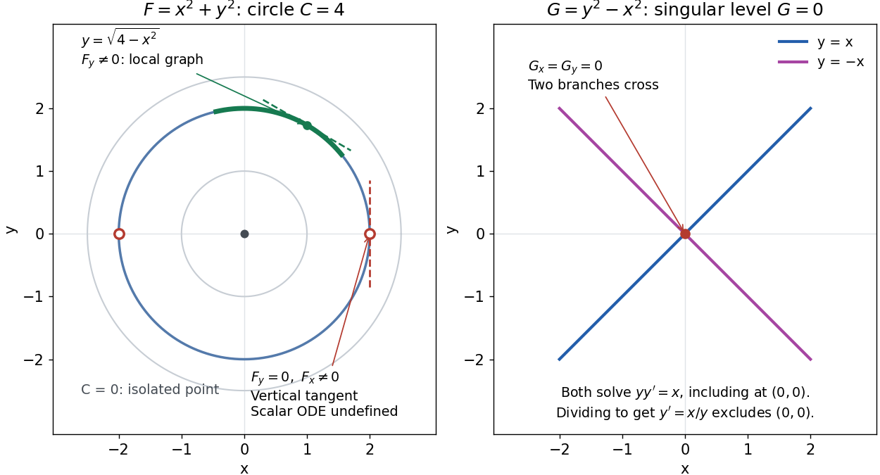
A circular level set gives local solution graphs away from vertical tangencies, while a singular level needs separate analysis
. Details. 
The precise local criterion uses the implicit function theorem. Let be continuously differentiable on an open subset of the plane, with . If its partial derivative , the nearby level set is a unique continuously differentiable function graph through that point. The chain rule givesThis proves that the local function graph solves there. For a different prescribed equation , one must also check along that branch and that it stays in the domain of . A level set by itself does not verify an arbitrary ordinary differential equation.[ref]
8.5 Inverse and implicit function theorems. §8.5.1, Theorem 8.5.6 and the preceding circle example: local existence, uniqueness and derivative of an implicit graph
For , the upper branch through has and tangent line slope . At , however, and . The circle remains a smooth regular level set with a vertical tangent line: it can be written locally as , but not as a single function graph over an open interval containing . Moreover, is undefined there, so the scalar solution of a differential equation cannot include this point in its domain. Changing the parameter draws the curve through the point but does not extend that scalar initial value problem.
When both partial derivatives vanish, even the geometry needs separate inspection. The level is an isolated point, not a function graph on any nonempty open interval. The zero level set of instead consists of the two lines and crossing at the origin, where . Each line satisfies the implicit ordinary differential equation , including at the origin; the explicit form excludes the origin. Thus algebraically dividing by a vanishing coefficient changes the domain and can change which solutions of a differential equation are admissible. Vanishing alone is only failure of a sufficient test: has the smooth zero function graph despite everywhere on it.
Implicit solutions are especially useful for exact first-order ordinary differential equations and for finding a first integral of an ordinary differential equation: a conserved relation can reveal allowed states without an explicit formula. For the normalized harmonic oscillator written as , , the energy has . Its positive level sets are the same circles. Where , eliminating time gives and the local implicit solution above. The harmonic oscillator's parametric curve continues through because its vector field governing evolution in time is defined there; treating as the independent variable fails at that turn. The origin is an equilibrium point of the harmonic oscillator, although it is excluded from the scalar equation .
Descending order statistics Created 2026-10-06 Updated 2026-10-07
Descending order statistics list a sample from greatest to least. If uses the usual increasing convention, then . This notation distinguishes the next-highest value used by revenue equivalence from the second-smallest sample value.
Field conjugate to an order parameter Created 2026-10-06 Updated 2026-10-20
A field conjugate to a scalar order parameter contributes to its free-energy density. Differentiating the equilibrium free energy with respect to gives , with density or extensive normalization stated consistently. In a ferromagnet the conjugate field is magnetic; for a fluid-density order parameter it is related to a chemical-potential difference. It can explicitly break the symmetry whose spontaneous breaking defines the ordered phase.
Altazimuth mount 2026-10-06
An altazimuth mount points an optical telescope using altitude and azimuth rotations. A mount restricted to elevations no greater than the zenith must change its azimuth by approximately half a turn when a target crosses the zenith.
Open-string endpoint momentum flux Created 2026-10-06 Updated 2026-10-14
For the Nambu-Goto phase-space action, with . Thus . Free endpoint variations force individually. A Dirichlet boundary condition allows an external support or D-brane to absorb momentum in the fixed direction.
Psi-ontic model 2026-10-06
An ontological model of a quantum system is psi-ontic if distinct pure states have mutually singular preparation distributions. The physical state then determines which pure quantum state was prepared, almost surely in the pairwise sense. Extra underlying variables may still exist. The PBR theorem establishes this conclusion under preparation independence and exact quantum predictions.
Psi-epistemic model 2026-10-06
An ontological model of a quantum system is psi-epistemic if some pair of distinct pure states has preparation measures with nonzero overlap. The same physical state can then be compatible with either preparation. This precise measure-overlap definition is stronger than merely interpreting a wave function as information or a computational tool.
Preparation independence 2026-10-06
Independently operated quantum state preparations are assumed to produce independent underlying physical states. Their joint preparation measure factors into the single-system measures. This ontic factorization is an additional assumption, not a consequence of operational independence alone. It turns a common single-system overlap of mass into a common -system overlap of mass in the PBR theorem.
Pusey-Barrett-Rudolph theorem 2026-10-06
Under preparation independence, an ontological model of a quantum system reproducing exact quantum quantum measurement probabilities cannot assign overlapping preparation measures to distinct pure states. An exclusion quantum measurement on independent copies makes every outcome impossible for one possible preparation; a common ontic region would require every response to vanish there. Thus the conclusion is a psi-ontic model, not a blanket exclusion of hidden variables or all informational interpretations.
Graph estimate for the harmonic oscillator 2026-10-06
For and smooth compactly supported , integration by parts givesDropping the nonnegative weighted derivative term proves the displayed bound. For a weak resolvent solution in the one-dimensional harmonic oscillator form domain, apply the bound to , where is a smooth cutoff. The cutoff error is bounded in L2 space and tends to zero. The Fatou lemma then shows that and belong to L2 space, identifying the strong operator domain.
For positive real with , minimizing gives with arbitrary . Around , the real scalar squared masses are , while the three Weyl spinor masses are . Their weighted supertrace vanishes. The massless is the goldstino; the two real modes form a tree-level pseudomodulus. The stability bound follows from , after minimizing the final square over .
Numerical radius Created 2026-10-06 Updated 2026-10-14
The radius is a scalar derived from the numerical range of an operator, rather than the range set itself.
For a bounded linear operator on a complex Hilbert space, the numerical radius is the supremum of the absolute values in its numerical range of an operator. It is a norm equivalent to the operator norm, with . For a self-adjoint operator the two norms agree.
Numerical-range spectral enclosure 2026-10-06
For a bounded self-adjoint operator, outside the closed numerical range yields . The same inequality for makes the range dense, and the first makes it closed. Thus is in the resolvent. The enclosure remains valid for general bounded Hilbert-space operators by the analogous adjoint numerical-range argument.
Matrix preconditioning Created 2026-10-06 Updated 2026-10-31
Matrix preconditioning transforms a linear system using an inexpensive auxiliary solve to improve its eigenvalues. For symmetric positive-definite matrices, a symmetric positive-definite matrix produces , preserving the symmetric structure needed by the conjugate gradient method.
A useful matrix preconditioner combines a cheap solve with favorable transformed eigenvalues; neither property alone is enough.[ref]
The aim is to make each correction more effective without making it expensive. The example under diagonal scaling for a two-dimensional linear system turns thin ellipses into nearly circular ones and makes preconditioned steepest descent effective.
Pure cubic number field Created 2026-10-06 Updated 2026-10-07
A pure cubic number field is a degree-three number field generated by a root of for a rational number that is not a rational cube. For a positive square-free integer , this polynomial is an Eisenstein polynomial at any prime dividing . The ring of integers of a number field depends on congruences at , as expressed by the integral basis of a nonexceptional pure cubic field.
Null-gradient affine-geodesic identity 2026-10-06
If is a null gradient, symmetry of the Hessian gives . Its integral curves are therefore affinely parametrized null geodesics, rather than merely null curves with a nonaffinity term.
Parallel auxiliary null vector 2026-10-06
For an affine null geodesic congruence with future tangent , choose a future unit timelike vector on a transverse section, put , and set there. It has and . Parallel transport along each generator preserves these contractions by metric compatibility and . The construction is local up to caustics and supplies the auxiliary normal for a screen-space projector.
There are unlisted articles, also show them or only show them.