
Past exam of the mathematics course of the University of Cambridge 2001 iii Paper 7 5 Solution Created 2026-10-03 Updated 2026-10-14
Let for a bounded normal operator on a nonzero complex Hilbert space. The zero Hilbert space has the trivial calculus. Take the inner product linear in its first argument. The continuous functional calculus is an isometric unital star-representation with . The Borel calculus will act on , the algebra of actual bounded Borel measurable functions. A quotient by null functions is introduced only after specifying the spectral measure; there is no preferred scalar measure such as plane area on .
Here is a construction that also covers a nonseparable Hilbert space. For , the positive functional has a finite regular Borel measure by the Riesz-Markov-Kakutani representation theorem. On continuous functions,Continuous functions are dense in . Hence extends to a unitary map from that space onto . This subspace reduces and , which correspond to multiplication by and . Decompose as an orthogonal direct sum of such cyclic reducing subspaces, using maximality: a nonzero vector in the remaining orthogonal complement would generate another summand. The family need not be countable. This is the cyclic multiplication model for a normal operator.
On each summand define to be multiplication by , for , and take their bounded direct sum. It defines a unital star-homomorphismThus , , and positivity of gives positivity of . The continuous functional calculus is recovered on .
Set for a Borel subset of . Then is an orthogonal projection, , , and disjoint countable unions add in the strong operator topology. Indeed on every multiplication summand the indicators add pointwise, and the tail squared norm is the measure of a decreasing sequence of sets tending to the empty set. Thus is a projection-valued measure, andFor , polarization gives scalar measures satisfying . Regularity of these finite scalar measures and uniqueness in the Riesz-Markov-Kakutani representation theorem make the projection-valued measure unique: its values on continuous functions determine all scalar measures and hence every projection. This also makes the calculus independent of the chosen cyclic decomposition.
The correct convergence assertion is bounded pointwise convergence in the strong operator topology. If pointwise and , thenby the dominated convergence theorem. This need not be convergence in operator norm. For multiplication by on , the functions converge pointwise to , their operators converge strongly to zero, but their operator norms are all one.
A Borel measurable function can vanish spectrally without vanishing pointwise. Precisely, if and only if for every , andThe upper norm bound follows by integrating against vector measures; a unit vector in any nonzero projection gives . The induced map on the quotient by these spectral-null Borel measurable functions is isometric. Every nonempty relatively open subset of has nonzero spectral projection, since otherwise a nonzero continuous function supported there would contradict faithfulness of the continuous functional calculus. This full support gives the usual continuous spectral mapping theorem, but for a Borel measurable function the exact statement is insteadIf an indicated neighborhood has zero projection, define a bounded reciprocal of off it and zero on it; the calculus supplies an inverse. Conversely unit vectors in the nonzero projections for arbitrarily small neighborhoods give arbitrarily small, contradicting invertibility. This is spectral essential range in Borel functional calculus. For example in the multiplication model on , although the pointwise range of that function is .
Spectral projections provide reducing subspaces, and : the squared norm of is . In finite dimension the calculus is simply , the sum over eigenspaces. In general it also permits discontinuous cuts and Borel choices of square roots, such as with , giving a normal operator with even when a continuous scalar branch is unavailable.
Any bounded operator commuting with both and commutes with their continuous functional calculus and with all . To justify the latter, regularity approximates by uniformly bounded continuous functions in the norms of any finite list of vector measures; the resulting net converges strongly to . Thus the Borel calculus lies in the Von Neumann algebra generated by . On a separable Hilbert space, a countable dense list of vectors gives a controlling measure ; spectral-null sets are exactly its null sets, and the range is the represented , equal to that Von Neumann algebra. Without separability this last equality is not automatic: for the diagonal operator with one eigenvector for each , the generated Von Neumann algebra has arbitrary bounded diagonal functions, while the original Borel calculus has Borel diagonal functions. The spectral-measure construction and the strong convergence theorem themselves require no separability. This distinguishes the Borel functional calculus for a normal operator from its continuous predecessor without confusing pointwise functions, spectral equivalence classes and topological closure.
Past exam of the mathematics course of the University of Cambridge 2001 iii Paper 7 4 Solution Created 2026-10-03 Updated 2026-10-14
The group consists of the nonvanishing continuous functions, and is a subgroup because multiplication is commutative: . The objective is a logarithm decomposition with finitely many integer obstructions, one for each bounded complementary component. No local connectivity of is assumed.
We use two elementary finite-neighborhood facts, which make the outline independent of the general Jordan theorem. Given a neighborhood of , take a finite grid neighborhood with . It can be chosen to be a finite union of polygonal surfaces with boundary. Its complement has finitely many bounded holes. Holes that lie in the same component of can be joined by thin polygonal corridors disjoint from , which are removed from . A hole lying in the unbounded component is similarly joined to the exterior. For the remaining finitely many components, corridors may be continued to include their chosen representatives . Small polygonal adjustments preserve and . Thus every remaining bounded hole lies in a distinct bounded component of and contains its representative. One may also arrange this for any prescribed finite list of bounded components by first keeping their representative points out of the grid neighborhood. All paths used are compact and disjoint from , so sufficiently thin corridors remain disjoint from .
For such a finite polygonal , winding indices identify the homology group with the free abelian group on its bounded holes. Here is a finite-chain explanation. Triangulate a large disc with as a subcomplex. Every integral one-cycle bounds a two-chain in the disc. Its filling coefficient is constant on each component of the complement of , is zero on the exterior, and is the winding index there. If all bounded-hole indices vanish, the filling is supported in , so the cycle already bounds in . Conversely the sum of the oriented faces in one hole has its chain boundary in and has index one in that hole and zero in the others. Thus cycles can be chosen with . These can be integral sums of boundary curves, which matters when components of are nested. This proves the needed statement using finite triangulation, not separation of an arbitrary simple closed curve. Together these are finite-hole neighborhoods of a planar compact set.
Now extend to a continuous near , using the Tietze extension theorem on its real and imaginary parts. Since , shrink the neighborhood until has no zeros, and choose within it as above. The winding of on the cycles defines integers . Setwhere only the finitely many represented holes are used. The winding of on every cycle of is zero. On each component choose a local complex logarithm at a base point and continue it along paths. Zero winding number around every loop makes the continued value independent of the path; local logarithm charts make it continuous. The continuous logarithm lifting criterion therefore gives on , and restriction gives . Thus , even when has infinitely many holes: each individual function uses finitely many factors.
To prove uniqueness, suppose a finite product equals on . Extend continuously to a neighborhood. There is close to after shrinking, so it has its small-branch logarithm. Hence itself has a continuous function giving a complex logarithm on that neighborhood. Choose there detecting all the finitely many as separate holes. Its dual cycles give , while a function with a logarithm has zero winding number. Therefore every . This proves both freeness of the listed rational functions and . All subgroups commute, soThis is planar logarithm factorization. If there are no bounded components the second factor is trivial.
For the Jordan curve deduction, let be homeomorphic to the circle. Parametrize it by with just the two endpoints identified. For , lift a logarithm of along the interval. Its endpoint increment is . The integer is additive, every integer is attained by a function with , and precisely when the lift descends to a logarithm on . Hence . The factorization says this is free abelian on the bounded complementary components; comparison of ranks, or tensoring with , shows that exactly one bounded component exists. There is also the unique unbounded component, so the complement has exactly two components.
We still need the common-boundary assertion. A proper closed arc has trivial exponential quotient because every nonvanishing function on an interval admits a logarithm. Factorization consequently makes the complement of such an arc connected, and since it is open it is path-connected. Fix and any neighborhood of , and choose a small open arc containing . The remainder is a proper closed arc. Join a point in each of the two complementary components by a path avoiding . This path must meet , and every such meeting lies in . The segment before its first meeting lies in the first region, and the segment after its last meeting lies in the second; continuity makes both regions meet . Thus every point of lies on both boundaries. Conversely either boundary is contained in the closed set . There are exactly two regions, one bounded and one unbounded, with common boundary , the Jordan curve theorem. This is Jordan separation from the exponential quotient; it does not assume the theorem in the factorization proof.
Past exam of the mathematics course of the University of Cambridge 2001 iii Paper 7 3 i Created 2026-10-03 Updated 2026-10-14
Past exam of the mathematics course of the University of Cambridge 2001 iii Paper 7 2 Solution Created 2026-10-03 Updated 2026-10-14
The exponential series is absolutely norm-convergent, since . Completeness defines the Banach algebra exponential . If , absolute convergence permits rearrangement of the product series, and the binomial identity givesTaking yields .
For the spectral hypothesis, put . Its complement has an open, hence path-connected, unbounded component containing . Join to an exterior point by a simple polygonal arc in that component, and continue it to infinity, avoiding . Removing this polygonal slit gives a simply connected open neighborhood of on which has a branch of the complex logarithm . The holomorphic functional calculus therefore defines and its composition rule givesThe relevant slit is chosen through the resolvent, not assumed to be a fixed negative-real-axis cut. This is the logarithm from a spectral slit in a Banach algebra.
Let be the subgroup of finite products of exponentials. It is a subgroup because and reversing a product gives its inverse. Each product is joined to by , so . Conversely, if , the convergent logarithm seriessatisfies , by the scalar analytic identity and functional calculus. Thus contains a neighborhood of . Its translates make open, and all other cosets are open too, making closed. Connectedness forces . Finally , so is normal. Thereforean open-and-closed normal subgroup. This is the identity component of Banach-algebra invertibles; finite products are essential and are not asserted to be single exponentials.
Past exam of the mathematics course of the University of Cambridge 2001 iii Paper 7 1 i Created 2026-10-03 Updated 2026-10-14
Past exam of the mathematics course of the University of Cambridge 2001 iii Paper 69 5 Solution Created 2026-10-03 Updated 2026-10-14
Interpret first as an infinitesimal screen area transported along generators of a future event horizon, not as the total area of an arbitrary trapped surface. Horizon generators form an affinely parametrized, hypersurface-orthogonal null geodesic congruence. The two-dimensional screen metric is positive definite. Its optical tensor has zero twist and decomposes asThe scalar here agrees with the supplied derivative definition: nullness and the affine geodesic equation remove the longitudinal terms in the contracted norm, leaving .
To derive the focusing equation, vary neighbouring geodesics and let be their screen Jacobi map. The geodesic deviation equation is , where . Hence satisfies . Taking its screen trace yields the Null Raychaudhuri equationSet . Since , the area-square-root optical focusing equation isThe PDF's plus sign before is inconsistent with its own positive shear definition. This is an actual source error, not an antisymmetrization or curvature-sign convention.
For an explicit check, take a flat-space twist-free beam with screen Jacobi factors and , for . ThenIts Ricci term is zero, so the result equals and has the opposite sign to the printed equation. This is flat-space anisotropic beam shear focusing.
Under the null convergence condition , the correct equation gives concavity of each local area square root. Equivalently . If a horizon generator had , integration gives a focal point within affine distance at most . Such a generator could not remain on an achronal boundary beyond the focal point. Under the usual global hypotheses that horizon generators remain regular and future complete, this contradicts their being generators of the event horizon. Hence and . Integrating over the horizon patches, and including newly joining generators which can add area, proves Hawking's area theorem. Global predictability/completeness assumptions are essential; the local differential inequality alone is not a theorem about arbitrary trapped-surface areas.
For the perfect fluid stress tensor, null contraction eliminates the pressure-metric term:A nonzero null vector cannot be orthogonal to a timelike fluid velocity. Thus the perfect-fluid null energy condition is preciselySeparate requirements or are not needed for this null focusing argument. With the Einstein equation, .
A cosmological constant contributes only a term proportional to , whose null contraction is zero:Therefore a nonzero cosmological constant does not change the fluid condition or the local area-focusing argument, though it can change the global asymptotics and which horizons and completeness hypotheses are appropriate.
Past exam of the mathematics course of the University of Cambridge 2001 iii Paper 69 4 Solution Created 2026-10-03 Updated 2026-10-14
Assume an asymptotically flat Reissner-Nordstrom spacetime, with , time normalized at infinity, and . PutNear , the Euclidean radial-time metric is . With , it becomesThe Euclidean black-hole regularity condition removes a conical defect only if has period . Therefore the Reissner-Nordstrom Hawking temperature isEquivalently this is the Reissner-Nordstrom horizon surface gravity divided by . The derivation assumes a nondegenerate horizon; the value zero at is obtained by the nonextremal limit, not by imposing conical regularity directly on the degenerate geometry.
For fixed nonzero , write . The horizon equation givesThe mass is increasing with , andThus the fixed-charge Reissner-Nordstrom temperature maximum occurs atThe curve starts at zero at , rises to this maximum, then falls as for large mass. During evaporation from , the mass moves from right to left: the temperature initially increases, reaches its maximum, and then decreases towards zero.
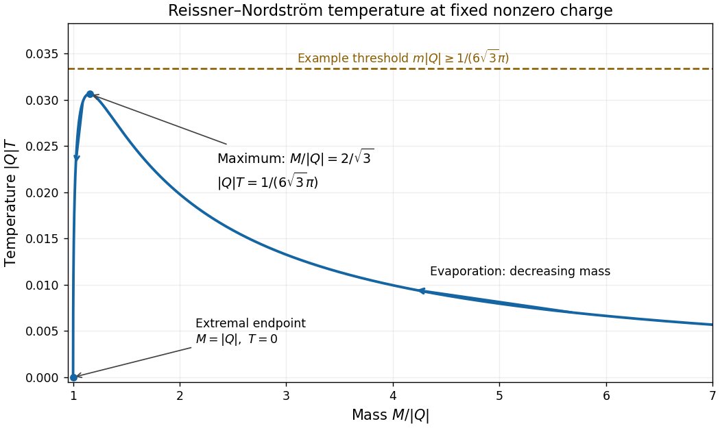
Reissner-Nordstrom temperature at fixed charge, its maximum and the evaporation direction
. Details. 
Under the printed thermal-emission cutoff, charged emission is absent throughout precisely when the entire mass path remains at or below the threshold:Equality is allowed because emission is assumed to require , not merely . The initial large mass ensures that the path includes the maximum.
With charge then conserved, neutral Hawking radiation lowers the mass until the system approaches the charge-preserving Reissner-Nordstrom evaporation endpoint:The limiting state is an extremal black hole, rather than a neutral zero-mass endpoint. Exact attainment in finite time is not established: near extremality , and the ideal radiation rate tends to zero. The conclusion is within the assumed thermal cutoff model, which omits nonthermal charge creation and other quantum corrections. For , the Schwarzschild temperature instead grows without bound in the extrapolated model, so no finite satisfies the stated all-the-way temperature bound.
Past exam of the mathematics course of the University of Cambridge 2001 iii Paper 69 2 Solution Created 2026-10-03 Updated 2026-10-14
The mass statement needs a nonzero parallel spinor and an isolated asymptotically flat spacetime; the zero spinor solves the equation on every geometry and cannot imply anything about mass. Assume the usual complete regular spin initial data and dominant energy condition used by the positive energy theorem, with the spinor tending to a nonzero constant at infinity. Let be its future causal Dirac current.
The Nester two-form can be written, up to normalization, asIt is bilinear in and . For a spacetime-parallel spinor it vanishes identically, and hence so does its asymptotic flux. The ADM boundary term of the Nester two-form identifies that flux, up to a fixed positive normalization, asThe positive energy theorem gives . Since is nonzero future causal, a future timelike ADM momentum would have strictly positive contraction with it. Consequently the ADM momentum is zero or null:In a rest frame, when one exists, this immediately says . The usual regular asymptotically flat rigidity conclusion also excludes a nontrivial null-momentum configuration and gives flat initial data. This is the spinorial boundary-charge proof, not an inference that every Lorentzian manifold with a parallel spinor is flat. Without the asymptotic and global hypotheses the local spinor equation alone does not define, let alone determine, an ADM mass.
For the modified connection, it is important to fix the Clifford algebra normalization. WriteThe compatible spinor curvature identity isIndeed, rescaling conventional gamma matrices by rescales by , while leaving the geometric spin connection unchanged. Since the connection is torsion-free and , the cross terms cancel in the modified commutator:Thus the Killing-spinor integrability with rescaled gamma matrices equation isA factor of two in the convention for antisymmetrization multiplies the whole zero equation and cannot change this relative coefficient.
The two printed coefficients are consistent with , namely . In that convention the displayed integrability equation becomes on each solution. With the customary convention , the coefficient is instead , and the final Ricci coefficient below is . The PDF does not state its Clifford normalization, so these alternatives must be distinguished rather than mixing them.
In four spacetime dimensions the complex Dirac spinor fibre has dimension four. Four independent solutions of span that fibre at every point: a solution vanishing at one point vanishes everywhere by parallel transport. Therefore the integrability matrix annihilates every spinor and is the zero matrix. The six bivector matrices are linearly independent, as is seen by taking traces against them; their trace pairing is a nondegenerate multiple of the metric on two-forms. Expressing therefore givesThis proves that maximal Killing spinors force constant negative curvature, not merely an Einstein Ricci tensor. Contracting in four dimensions givesFor this is the requested Einstein equation. Since , its Ricci tensor automatically has rank four; under the maximal-spinor hypothesis the additional rank assumption is redundant. If the stated four-dimensional solution space is interpreted directly as the pointwise kernel of the algebraic integrability equation, the same spanning and trace argument applies.
There are unlisted articles, also show them or only show them.