Gauss's law relates the electric field on a closed surface to the net electric charge inside it. In SI units, with outward unit normal ,Here describes a volume charge density, and is the vacuum permittivity; for ideal point or surface charges, use the enclosed electric charge directly rather than an ordinary volume-density integral. The left side is electric flux: the surface integral of the outward normal component of the electric field. Field directed outward contributes positively; field directed inward contributes negatively. The equality uses net signed electric charge, so positive and negative enclosed charges can cancel. The Gaussian surface is an imagined accounting boundary, not necessarily a material object. See OpenStax, explaining Gauss's law.
Where the electric field and charge density are smooth, the local statement is . The divergence theorem connects this divergence to the surface integral. This is the satisfying connection between local sources and global accounting: a surface can register how much net electric charge it encloses without revealing where that charge is located within it. A point charge requires care with the singular field at its position; the integral formulation remains useful with a boundary that avoids the charge.
The law fixes total electric flux, rather than every value of the electric field. In an uncharged region, a uniform electric field crosses a cube of side . Its left and right faces contribute and ; the other four faces contribute zero. Thus the net electric flux is zero while the electric field is nonzero everywhere. Charges outside a Gaussian surface can change the field on it without changing its net electric flux. Conversely, fields cannot generally be reconstructed from enclosed electric charge alone. Electrostatics also requires the electric field to be the negative gradient of an electric potential, with appropriate boundary information. This distinction is emphasized in Feynman lectures II.5, application of Gauss' law.
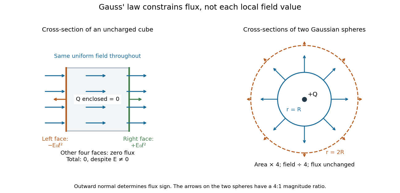
Zero net flux can coexist with a nonzero uniform field, and equal enclosed charge can give different field magnitudes on different spheres
. Details. Spherical symmetry supplies the extra information needed for a particularly simple calculation. An isolated spherically symmetric charge distribution in vacuum produces a radial electric field, constant in magnitude on each concentric sphere. Its electric flux is therefore , givingOutside the distribution, doubling quadruples the surface area and divides the radial electric field by four, while the electric flux stays . The inverse-square dependence is an area-dilution result. The electric field of a uniformly charged ball and electric field of a uniformly charged spherical shell show that the same total charge can give different interior fields. These symmetry arguments and their limits are developed in OpenStax, applying Gauss's law.
In macroscopic matter with free charge density and free current density ,The electric displacement and magnetic field strength encode the material response.
These are the Maxwell equations after separating free and bound material sources.
Past exam of the mathematics course of the University of Cambridge by  Codex 0 Created 2026-09-24 Updated 2026-10-07
Codex 0 Created 2026-09-24 Updated 2026-10-07A probability-preserving bijection pairs outcomes of two events without changing their masses, proving the events have equal probability.
Structural induction proves a property of every recursively generated object by checking the initial objects and showing that every construction rule preserves the property.
A counterexample is one instance satisfying a claim’s hypotheses but not its conclusion, and therefore disproves the universal claim.
First-order logic permits quantification over elements of a structure while its nonlogical symbols describe operations, constants, and relations.
Propositional logic studies reasoning with whole propositions represented by letters such as and , and propositional formulas built from them using logical connectives. The classical two-valued, truth-functional presentation below assigns each primitive proposition either true or false: each compound value depends only on its component values. This is classical propositional logic; other systems, including Intuitionistic propositional logic, have different semantics and rules.
Starting with and , one can build by logical negation, by logical conjunction, by logical disjunction, and by logical implication, then combine these into larger propositional formulas. Parentheses specify the construction: has logical conjunction as its outermost logical connective. Primitive propositions have no internal structure in this language; a first-order formula can additionally describe objects and quantify over them. The formation rules are given in forall x: Calgary, chapter 6.
The following truth table shows the four basic logical connectives. Logical disjunction is inclusive: is true when either or both inputs are true. Classical logical implication has exactly the same values as ; its only false row has true and false. These truth conditions are specified in forall x: Calgary, chapter 9.
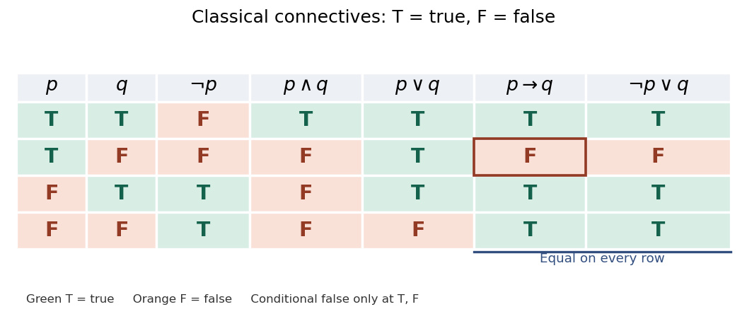
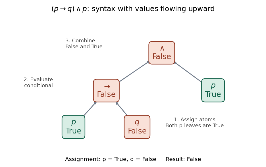
Evaluate from the inside out: first the logical implication, then the outer logical conjunction. The final column also tests the logical implication expressing the modus ponens rule:At , the logical implication is false, so the logical conjunction is false. The abstract syntax tree below separates the construction of the propositional formula from the values propagated through it. Both occurrences of receive the same value from the Boolean valuation. With the opposite assignment , the logical implication is true but the logical conjunction is still false because its second input is false. Recursive evaluation and exhaustive truth tables are explained in forall x: Calgary, chapter 11.


The last column is always true: is a tautology. This expresses the logical validity of the modus ponens rule: whenever both premises and are true, is true. It does not say the premises are true under every Boolean valuation; their logical conjunction is true only on the first row. For a short natural deduction proof outline, assume , extract both conjuncts, apply the implication elimination rule to obtain , then discharge the assumption by the implication introduction rule. See forall x: Calgary, sections 17.3–17.5.
Three tests answer different questions: Boolean satisfiability requires at least one true row, a tautology requires every row true, and a contradiction has every row false. Thus is a tautology, is a contradiction, and is satisfiable but not a tautology: it is true only at . See forall x: Calgary, sections 12.1–12.4.
Propositional logic is useful because an inference pattern can be checked once and reused for many choices of propositions. Its beauty is that a finite truth table completely settles classical truth-functional questions about a fixed propositional formula. But logical validity does not verify real atomic claims. If means “the switch is closed” and means “the lamp is lit”, a valid use of the modus ponens rule still requires establishing its premises about the apparatus; the truth table supplies neither an observation nor a causal explanation. See forall x: Calgary, chapter 2 and chapter 10.
Backward induction proves or computes a finite sequence of statements by starting at its terminal index and stepping toward the initial index.
An American option may be exercised at any time up to maturity. Its value is the Snell envelope of its discounted exercise payoff.
In the Black-Scholes model with constant interest rate and volatility , a risky asset satisfiesunder the risk-neutral measure.
In a finite market, absence of arbitrage is equivalent to the existence of an equivalent martingale measure. If that measure is unique, every contingent claim has a unique no-arbitrage price given by its discounted expectation.
At each node a positive stock price moves to or , with , while a bank account grows by a fixed gross factor . Assume both successors have positive physical probability, no dividends, a frictionless market with no trading costs, divisible holdings, unrestricted short selling, and borrowing and lending at the same fixed . A self-financing portfolio receives no outside cash after its initial funding; subsequent rebalancing uses its own proceeds.
This binomial market excludes arbitrage exactly when . If , borrowing to buy one share gives terminal gains or ; these are nonnegative and one is positive. If , short selling one share and lending its proceeds gives the analogous arbitrage. Strict inequalities allow a positive risk-neutral probability for each state. The two traded payoffs also span both successor states, giving market completeness relative to the information generated by this tree.
For independent return innovations and a predictable process of holdings , wealth obeysThe investor chooses the holdings to maximize expected utility of terminal wealth.
In expected-utility portfolio choice, an increasing utility function prefers greater wealth, while concavity models aversion to risk.
A utility function assigns numerical values to outcomes consistently with preference comparisons. It represents utility; the representation and the preference concept are distinct.
An arbitrage is an allowed self-financing portfolio with zero initial wealth, nonnegative terminal portfolio wealth almost surely under the physical probability measure , and strictly positive terminal wealth with positive probability. In a finite model where every state has positive probability, nonnegativity means no loss in any state. Positive expected return alone does not establish arbitrage: losses may still occur.
For the binomial market example, suppose the European call option sells for 13 while its replicating portfolio costs . Sell the call, buy its replicating portfolio, and lend the surplus in the bank account. The initial net cost is zero. At maturity the call obligation and portfolio cancel in either state, leaving . A price below permits the reversed construction, using short selling and borrowing. This is the law of one price made operational; the assumed trading permissions are essential.
There are unlisted articles, also show them or only show them.