
Linear operator theory studies linear maps, their spectra, invariant subspaces, and normal forms such as Jordan normal form. In a finite-dimensional vector space, eigenvalues identify parameters for which a shifted linear operator cannot be inverted. In an infinite-dimensional vector space, inversion can fail even without an eigenvector. The spectrum of a bounded operator captures this larger obstruction and connects linear algebra with the approximation questions of functional analysis.
For an -by- square matrix over a field, its matrix trace is the sum of its diagonal entries:For example, has trace . Adding corresponding diagonal entries immediately proves linearity:Thus matrix trace is a linear functional on the vector space of -by- matrices.[ref]
Linear Algebra Done Right by Sheldon Axler (4th edition). Axler, Linear Algebra Done Right, fourth edition, §8D, definition 8.47 and result 8.56
The surprising point is that the sum is intrinsic to a linear operator, even though individual diagonal entries depend on the basis. The cyclic property of the trace gives, for any invertible matrix ,Hence matrix similarity preserves trace. For the example above, choose the change-of-basis matrix . ThenThe diagonal entries have changed but their sum has not. This makes trace useful for extracting a feature of the underlying linear operator without finding a preferred basis.
Over the complex numbers, or over the real numbers after allowing complex eigenvalues, the trace equals their sum with algebraic multiplicity:No diagonalizable matrix hypothesis is needed.[ref]
Linear Algebra Done Right by Sheldon Axler (4th edition). Axler, Linear Algebra Done Right, fourth edition, §8D, results 8.50–8.52
To see why, use triangularization over an algebraically closed field: an upper triangular matrix similar to has the eigenvalues on its diagonal, counted with algebraic multiplicity, because its characteristic polynomial is . Similarity preserves trace, so summing that diagonal proves the formula.For instance,There is only one independent eigenvector, since , so is not a diagonalizable matrix. Nevertheless its repeated eigenvalue contributes twice. For our earlier , the characteristic polynomial is , its eigenvalues are and , and their sum is . An inexpensive diagonal sum therefore gives spectral information before solving the characteristic polynomial.
The trace of a real matrix does not give that linear map's volume factor: that factor is the absolute value of its determinant. For example, has trace and area factor , but has trace and volume factor . Their occasional numerical agreement in two dimensions is a coincidence. The connection between trace and local volume change gives a geometric interpretation near the identity matrix, and describes the volume rate of a flow map generated by a linear system of differential equations.
For an -by- square matrix over a field, its matrix inverse is an -by- matrix satisfying both identitieswhere is the identity matrix. It exists exactly when is an invertible matrix, equivalently when its matrix rank is or its determinant is nonzero. It reverses the linear map: applying and then recovers the input, while applying and then recovers the output.[ref]
https://ocw.mit.edu/courses/18-06-linear-algebra-spring-2010/resources/lecture-3-multiplication-and-inverse-matrices/. Strang, MIT 18.06 Lecture 3: the two inverse identities
The matrix inverse is unique. If and both satisfy the identities, then . Although the definition is two-sided, for finite square matrices either identity alone suffices: forces a trivial kernel, whereas forces surjectivity; either makes an invertible matrix by the rank-nullity theorem. Rectangular matrices may have only one of these properties.
For a concrete example, takeDirect matrix multiplication givesConsequently the vector follows a reversible journey:The columns and are the images of the standard basis vectors. They turn the unit square into a parallelogram; the matrix inverse restores both the square and its surrounding grid. Since , this example changes shape while preserving area, illustrating that invertibility does not require preserving lengths or angles.
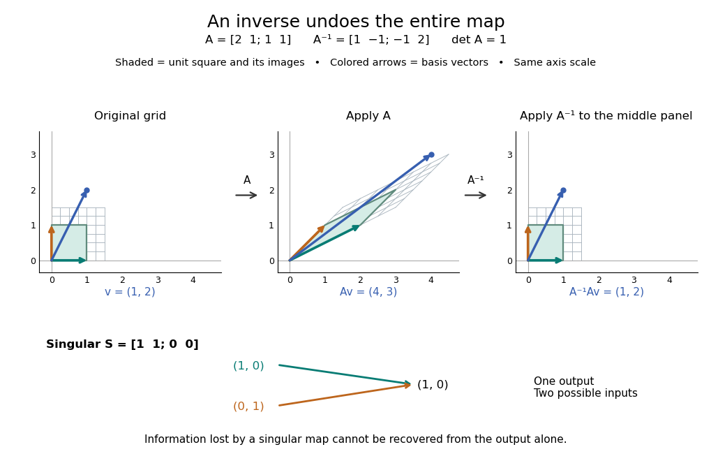
For comparison, the singular matrixcannot have a matrix inverse: the output cannot specify which of the two inputs occurred. Their difference belongs to its kernel. Indeed collapses the plane to a line, its matrix rank is one, and its determinant is zero. No subsequent function of the output alone can reconstruct every input.
An important use of the matrix inverse is describing the unique solution of a linear system:For , the preceding computation solves and , giving . In computation, usually solve the linear system using Gaussian elimination and a factorization such as an LU decomposition, rather than forming every entry of the matrix inverse. The inverse formula specifies the answer; a factorization provides a reusable way to compute it for each right-hand side.[ref]
https://www.mit.edu/~18.06/Spring17/final-sol.pdf. MIT 18.06, Spring 2017 final solutions, problem 5(b): solve with triangular factors rather than computing inverses
Here the LU decomposition is especially simple:Solve by forward substitution in a triangular system: and . Then solve by backward substitution in a triangular system: and . The same factors work when changes. If the whole matrix inverse is actually needed, its th column is the solution of , where is the th standard basis vector.
Reversing several operations means undoing the last one first. For invertible matrices of the same size,because , and the product in the other order is also . This is why a change-of-basis matrix uses its matrix inverse to reverse the direction of coordinate conversion.
For an invertible matrix and real vectors , the matrix determinant lemma statesThe expression is a scalar, so a rank-one matrix update changes the determinant by a single multiplicative factor. One need not expand the updated determinant entry by entry.
For the preceding example with , the dot product is . Hence the updated determinant is . Direct evaluation confirmsMore generally, let for a real scalar . The same calculation gives . The determinant is one at , two at , and zero at .
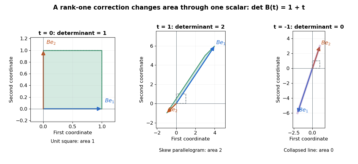
A compact proof explains the scalar reduction. Put and factor . If , choose a basis starting with . In that basis, , while every other basis vector changes only by a multiple of . Its matrix is triangular with diagonal , giving the required determinant. If , the correction vanishes. This uses multiplicativity of the determinant to restore the factor .
The denominator in the Sherman–Morrison formula is exactly this factor. The rank-one update singularity criterion therefore identifies when the updated matrix inverse ceases to exist. Batson, Spielman and Srivastava use both identities for the symmetric update in Twice-Ramanujan Sparsifiers, section 2.3, Lemmas 2.1–2.2.
The dual space of a vector space over a field is the vector space of all linear functionals . Think of a vector as an input and a linear functional as a scalar-valued measurement of that input. For , the rules , , and are different elements of the dual space. None needs a notion of length or angle.
Its operations combine measurements pointwise:The dual basis explains the finite-dimensional structure: specifying a linear functional's values on a basis determines its value on every vector. Thus an -dimensional vector space has an -dimensional dual space. The spaces have the same dimension, but their elements play different roles: an input and a rule that measures an input. [ref]
Linear Algebra Done Right by Sheldon Axler (4th edition). Axler, Linear Algebra Done Right, fourth edition, §3F, definitions 3.109–3.112
.This separation is useful when changing coordinates. The dual pairing must stay the same while the component lists for and change in opposite ways. Covector transformation under a change of basis makes the compensation explicit. An inner product on a finite-dimensional real vector space gives one way to represent each linear functional by a vector, but that representation uses the chosen inner product; the dual space itself does not require one.
Here dual space means the algebraic dual: all linear functionals. For a topological vector space, the continuous dual space keeps only the continuous linear functionals. In infinite dimension, this can be a proper vector subspace; discontinuous functional detected by vanishing sequence tails gives an example. The distinction matters when a scalar-valued measurement must respond continuously to small input changes.
The kernel of a linear map is the vector subspace of inputs sent to zero. Linearity makes it a vector subspace: if , then for all scalars . A vector in the kernel represents a change that the map cannot detect, since for every input .
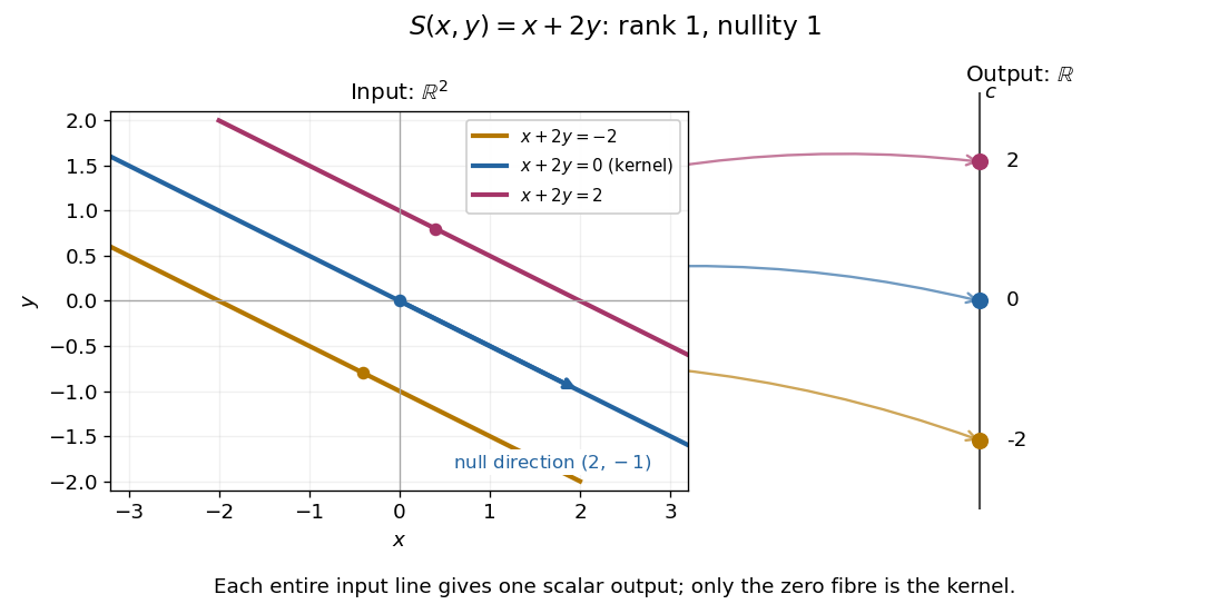
For given by , the zero-output equations are and . ThusIncreasing the first input while decreasing the second by the same amount leaves the output unchanged. For the linear functional , the kernel is the straight line shown in its diagram. A linear map is injective exactly when its kernel is the zero vector subspace, because is equivalent to .
The kernel describes invisible changes, rather than all inputs that produce a specified nonzero output. If , the corresponding fiber of a function is the affine solution space of a linear equation . The difference of two inputs in that fiber belongs to the kernel; an input in that fiber need not. In particular, for the fiber cannot be a vector subspace, since it does not contain the zero vector.[ref]
Solution Sets. Margalit and Rabinoff, Interactive Linear Algebra, §2.4.2, Key Observation and Remark: translate the homogeneous solution set by any particular solution
For the linear functional , , the kernel is . Each fiber is the parallel straight line . The input vector space is two-dimensional, but the output is one scalar: a whole straight line of inputs collapses to one point of the output real line.
An -by- square matrix over a field is invertible when it has a two-sided matrix inverse. Equivalently, its linear map is a bijection: every output comes from exactly one input. For a square matrix, the following conditions are equivalent:Here matrix rank means both full column rank and full row rank. The square hypothesis matters: a rectangular matrix can have full column rank without reaching every output, or full row rank without determining every input.[ref]
https://ocw.mit.edu/courses/18-06-linear-algebra-spring-2010/resources/lecture-3-multiplication-and-inverse-matrices/. Strang, MIT 18.06 Lecture 3: multiplication and inverse matrices
The equivalences explain why invertibility is a question about retaining information. A trivial kernel makes the linear map injective; the rank-nullity theorem then gives matrix rank , so its columns form a basis and the linear map is also surjective. Assigning to each output its unique input gives a linear map: the preimage of is . The determinant is nonzero precisely when the columns are linearly independent. Thus algebraic solvability and independent directions describe the same phenomenon; over the real numbers, nonzero oriented volume supplies its geometric interpretation.
A circulant matrix applies the same rule at every position of a finite ring: moving both the input and output indices one step leaves its entries unchanged. Its first column determines the whole matrix. For a length- vector , index rows and columns by and defineThe indices use modular arithmetic. Thus each column is the previous column shifted down one place, with the last entry wrapping around to the top. Multiplication is exactly circular convolution:This makes a circulant matrix a natural model for a periodic finite difference rule or a filter acting on a periodic record. Strang's MIT lecture develops this connection between circulant matrices, circular convolution and the discrete Fourier transform.[ref]
For example, the first column givesHere the indices wrap around modulo four. Each output compares a value with its two neighbors; this is the Graph Laplacian of a four-vertex cycle graph. A constant input gives zero, while an alternating input gives a large response. The Fourier diagonalization of a circulant matrix makes this distinction exact: its four eigenvalues are .
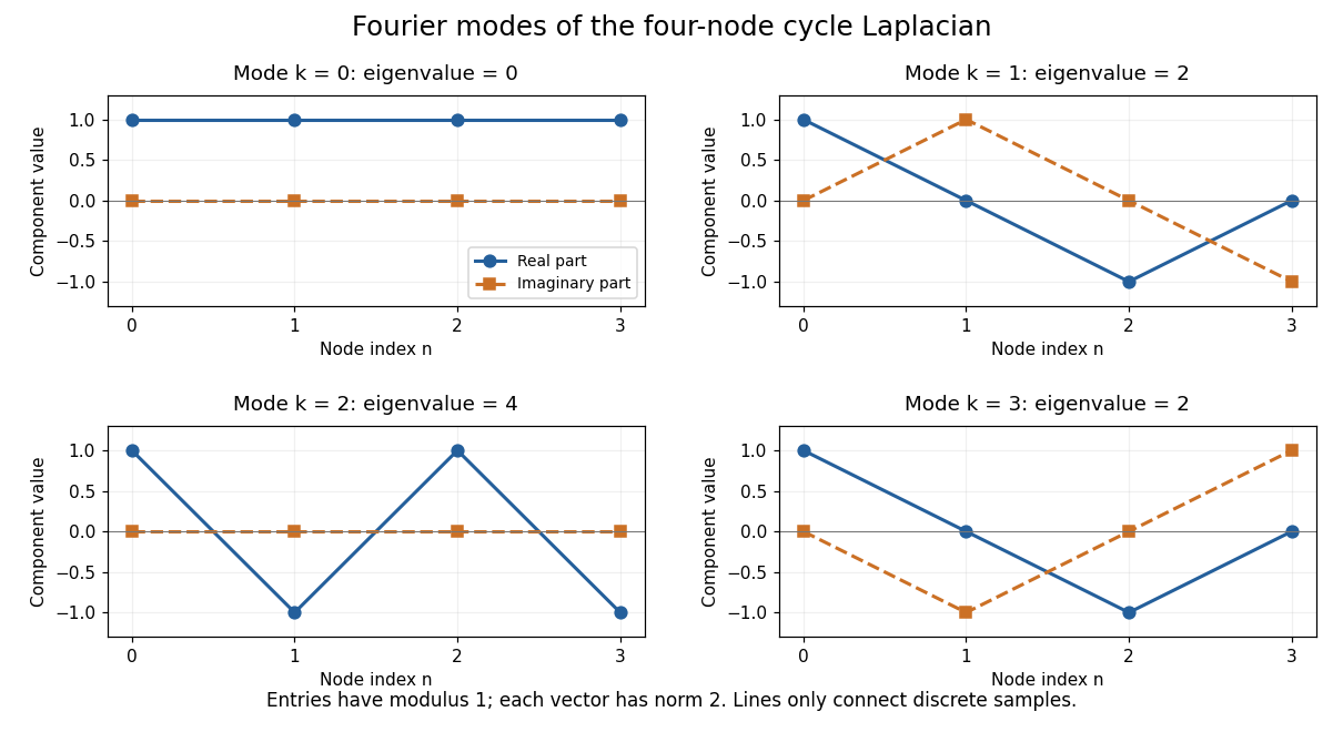
Fourier eigenvectors of the four-point cycle Laplacian
. Details. The plotted discrete Fourier modes are complex vectors, shown through their real and imaginary parts. Each entry has modulus one; the Euclidean norm of each length-four vector is two. In particular, modes and have the same real part but opposite imaginary parts, so they are distinct eigenvectors with the same eigenvalue.
The useful surprise is that every length- circulant matrix shares the same basis of eigenvectors, whatever its first column. One change of basis therefore simplifies an entire family of linear maps, instead of requiring a separate eigenvalue computation for each one. Bamieh's tutorial develops the discrete Fourier transform from precisely this simultaneous diagonalization problem.[ref]
https://arxiv.org/abs/1805.05533. Bamieh, Discovering Transforms: A Tutorial on Circulant Matrices, Circular Convolution, and the Discrete Fourier Transform (2018; revised 2022)
A change of basis rewrites a vector using a different ordered basis of the same vector space. The vector stays fixed; its coordinate vector changes because the measuring directions change. Both bases must describe every vector uniquely, so a change of basis is reversible.
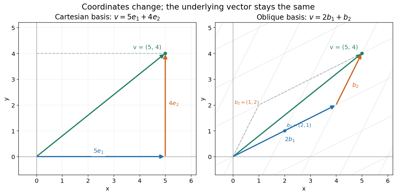
Start with the Cartesian basis , , and choose the new basis vectors and . For the vector ,The second coordinate vector says to travel once along and once along . Their vertical contributions cancel, leaving exactly the original horizontal arrow. The diagram shows two descriptions of that same arrow, with the same origin and endpoint.
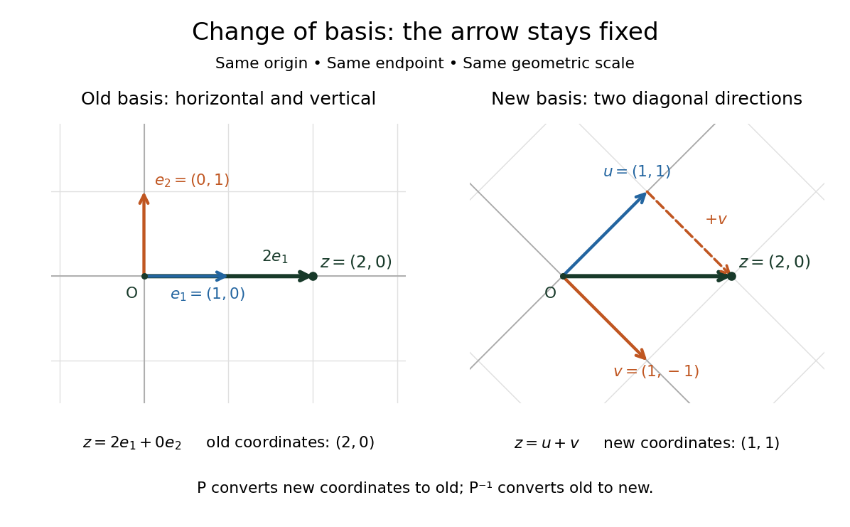
Choosing a useful basis can reveal simple structure hidden by the old coordinate vectors. Here the new basis describes common and opposing contributions. For two equal measurements , the new coordinate vector is : only the common contribution is present. In larger examples, a suitable basis can concentrate important information into a few coefficients. Strang's lecture on change of basis develops this principle through applications: the reversible change of basis preserves information, while subsequently discarding small coefficients loses information.[ref]
A unimodular matrix is a square integer matrix whose determinant is or . The decisive property is that its inverse matrix also has integer entries: multiplication by gives a bijection of the integer lattice onto itself. Thus an invertible linear map can preserve not only real coordinates but the requirement that every coordinate is an integer. These matrices form the integral general linear group.[ref]
Lecture 1: Introduction. §7, Definition 11 and Lemma 12, printed p. 9: determinant and integer-inverse characterization
For an original two-dimensional example, takeIts determinant is one, and it maps to . Conversely, the integer point comes from . For instance, has new coordinates relative to the columns and . No integer point disappears, although the basis vectors and their fundamental cell change shape.
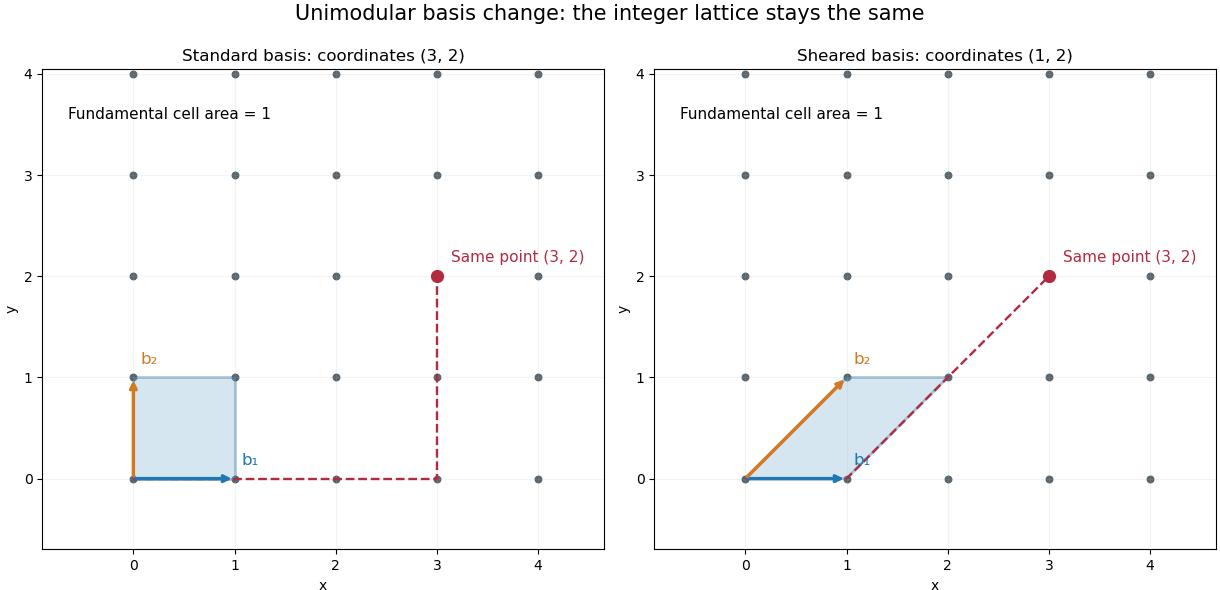
Two lattice bases generate exactly the same integer points
. Original drawings of the standard basis and the columns of . Both displayed cells have area one. The point has coordinates in the standard basis and in the sheared basis. Details.This is useful whenever coordinates must remain integral. A unimodular change of lattice basis can give a shorter or more convenient description without changing the objects represented. Smith normal form and Hermite normal form use controlled integer operations to simplify integer matrices; ordinary Gaussian elimination may divide by numbers that destroy integrality. The geometric freedom is substantial: a sheared basis may look completely different while describing exactly the same infinite set of integer points.
A determinant of is allowed too. Swapping two basis columns reverses orientation while preserving the integer lattice. The condition is therefore preservation of the complete integer structure, rather than a requirement to preserve orientation.
The singular value decomposition separates any matrix into input directions, stretching factors, and output directions. Every complex matrix admitsHere are unitary matrices, is the conjugate transpose, and is a rectangular diagonal matrix. Its diagonal entries are the singular values, ordered . We use the conventional letters: contains the right singular vectors , while contains the left singular vectors . Writing instead merely swaps these two matrix names; it requires swapping their roles consistently. For real matrices, choose orthogonal matrices and replace the conjugate transpose with the transpose.[ref]
Reading from right to left, expresses the input in an orthonormal basis, stretches or annihilates those coordinates, and assembles the output in another orthonormal basis. Unlike matrix similarity, the input and output bases can differ, and even have different sizes. A matrix has full factors of sizes , , and . If its matrix rank is , one can retain only the active columns, giving sizes , , and for ; the full additionally describes an unused output direction.
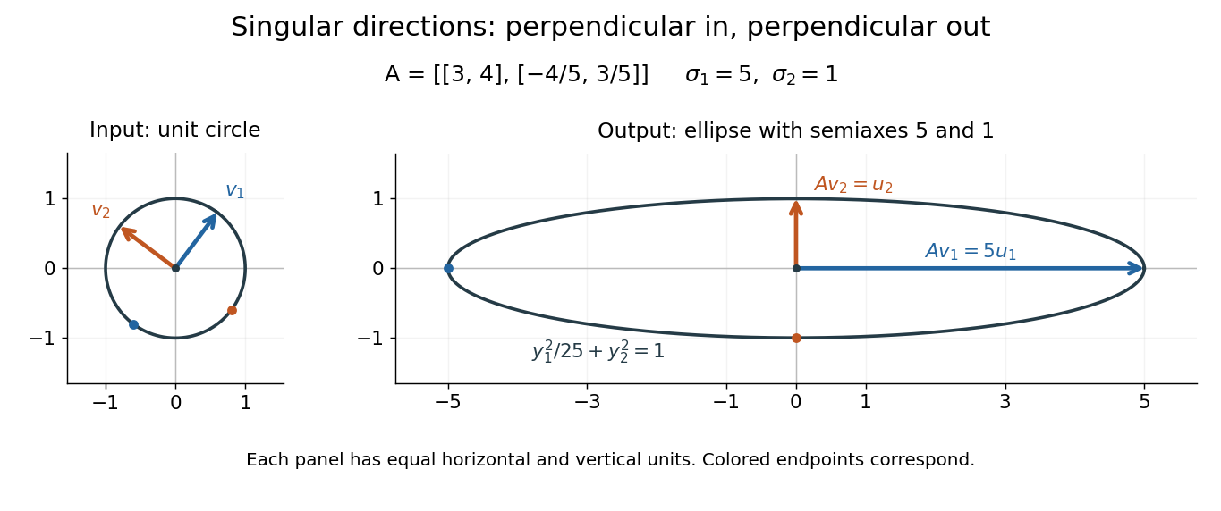
For a fully computed nonsymmetric example, takeMultiplication gives . The right singular vectors are and ; their images are and . Thus, parametrizing the unit circle by gives . Its image is the ellipse . The two singular values are its semiaxis lengths, and the left singular vectors point along its axes. The singular value decomposition finds precisely the perpendicular input directions whose images stay perpendicular.
For compression, write the matrix as a sum of outer products and retain the largest terms:where is the matrix rank. Among all matrices of matrix rank at most , minimizes the Frobenius norm error; this is the Eckart-Young-Mirsky theorem. The operator norm error is for . These statements concern specified norms, rather than guaranteeing that discarded details are visually or scientifically unimportant.[ref]
Consider an brightness matrix , withand , . The broad bright patch and alternating checkerboard have orthogonal row and column directions: . Their singular values are and . This low-rank approximation keeps the first outer product, giving , with Frobenius norm error and relative error . For example, becomes , and becomes : every entry changes by in magnitude. The discarded pattern is small but entirely lost.
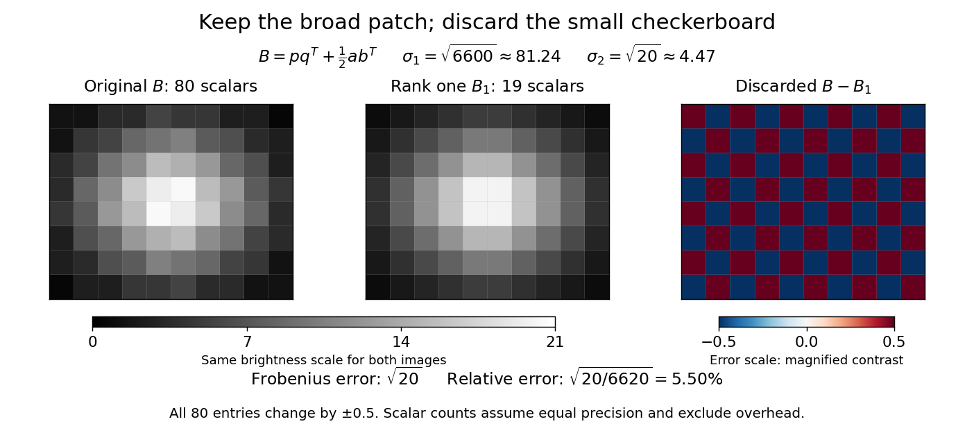
For this illustrative image compression, storing one normalized left singular vector, one normalized right singular vector, and one singular value requires scalars instead of . This counts scalars at equal precision, before storage overhead. In general, scalars beat only for sufficiently small , and small error requires a small discarded sum of squared singular values. The usefulness comes from measuring the tradeoff before throwing information away.[ref]
https://math.mit.edu/~gs/linearalgebra/ila5/SVD_Slides.pdf. Verma, Singular value decomposition of real matrices, slides 9 and 15–16
A vector space over a field is a set equipped with vector addition and scalar multiplication satisfying the vector space axioms. Its vectors can represent directed displacements, lists of measurements, polynomials, or entire functions. The common structure is that adding two elements and multiplying an element by a scalar remain meaningful operations inside the same space.
For example, uses coordinatewise addition and scaling. Withwe have . Moving twice along and once along reaches the same vector as five horizontal and four vertical steps. The two descriptions refer to different bases of the same space. A basis makes such descriptions unique; a spanning set makes them possible.


The space of real polynomials of degree at most two has basis : the polynomial is the linear combination with coordinates . The zero vector here is the zero polynomial, and addition combines coefficients. A derivative is a linear map on this space; its matrix records how it acts on the three basis vectors. The same coordinate machinery therefore handles both geometric motion and operations on functions.
The choice of field matters. The complex numbers form a one-dimensional vector space over with basis , but a two-dimensional vector space over with basis . The question "how many independent directions?" has an answer only after the allowed scalars are specified. Likewise, polynomials of degree exactly two do not form a vector space: subtraction can remove the leading term, and the zero polynomial is absent.
The usefulness of the abstraction is that a linear map is determined by its values on a basis. Once those images are known, linear combinations give its action on every vector. The rank-nullity theorem relates the number of attainable outputs to the number of invisible input directions, while change of basis lets us choose coordinates suited to the problem. Eigenvectors, for example, choose directions on which repeated application of a linear operator becomes scalar multiplication.
A historical source is Hermann Grassmann's Die lineale Ausdehnungslehre (1844). Its full title advertises applications to other branches of mathematics, statics, mechanics, magnetism and crystallography; the original edition is digitized by ETH-Bibliothek. This gives an early setting for treating geometric quantities algebraically across different applications, rather than attributing the modern axiom list to that title alone.[ref]
https://www.e-rara.ch/zut/content/titleinfo/1169335. Grassmann, Die lineale Ausdehnungslehre, Leipzig, 1844; ETH-Bibliothek Rar 5128
A sesquilinear form on a complex vector space is a map which, with the convention used throughout this article, is a linear map in its first argument and a conjugate-linear map in its second. For vectors and complex numbers , the defining identities areThe bars denote complex conjugation. No symmetry or positivity is required. Some authors choose the opposite convention; every formula here keeps the first argument linear.[ref]
For a basis of a finite-dimensional vector space, write , , and . Expanding by the two identities givesEvery complex matrix gives a sesquilinear form this way. The superscript means transpose, not conjugate transpose. Equivalently, the scalar is , where . This is the convention used for the matrix of a Hermitian form when symmetry is imposed. The coordinate formula follows directly by expanding the basis coefficients.[ref]
https://sites.math.washington.edu/~burke/crs/554/lectures/b-lecture4.pdf. Burke, Linear Analysis, Lecture 4, coordinate expansion for sesquilinear forms
For a concrete example on , let . Its matrix is : but , so it is not a Hermitian form. Also , so even real diagonal values cannot be assumed for an arbitrary sesquilinear form. By comparison, the bilinear form satisfies and has ; it cannot supply positive squared lengths on this complex vector space.
The effect of changing the complex argument of a multiplier is particularly revealing. For real numbers , sesquilinear forms satisfyThus a common change of complex argument cancels from the diagonal, whereas the two arguments rotate the output in opposite directions. Conjugating one argument is what replaces the scaling of a bilinear form by the nonnegative scaling needed for a Hermitian inner product. This mechanism also works in function spaces: for complex continuous functions on , obeys the same identities, letting integration measure overlap rather than merely multiply coefficients.
A bilinear form takes two vectors in a vector space over a field and returns a scalar in . Its defining property is separate linearity: holding either input fixed gives a linear functional of the other. For scalars and vectors ,This is a scalar-valued bilinear map; the chosen field is part of the definition.[ref]
Separate linearity does not mean that is a linear map on the vector space with componentwise vector addition and scalar multiplication. Over the real numbers, , whereas a linear map on the pair would give . The simplest example is on the one-dimensional vector space : fixing gives , but doubling both and quadruples their product.
A bilinear form measures how two inputs interact. The dot product measures alignment; a symmetric bilinear form can describe a quadratic form; an alternating bilinear form can measure signed area. A nondegenerate bilinear form turns each vector into a unique linear functional and so connects geometry with the dual space. The same short definition therefore supports lengths, bilinear orthogonal complements, and symplectic vector spaces, depending on the additional properties imposed.
Over the complex numbers, a bilinear form is linear in both inputs without conjugating either scalar. A Hermitian form instead is a sesquilinear form and conjugates when its inputs are exchanged. For complex matrices, the adjoint used with Hermitian forms and matrix C-star algebras is the conjugate transpose, whereas a bilinear form uses the ordinary transpose . For example, has , while the Hermitian form has .[ref]
Bilinear Forms by Keith Conrad. §1: examples and the Hermitian distinction
A Cartesian basis is an ordered basis of unit vectors along the mutually perpendicular axes of a Cartesian coordinate system. It is an orthonormal basis of a real Euclidean space: , with the Kronecker delta. In the plane, the familiar standard basis is , ; the vector is . A rotated pair of perpendicular unit vectors is also a Cartesian basis, even though its basis vectors have different standard basis entries.
The advantage is that coordinates can be measured separately by dot products, and the squared norm is the sum of their squares:These are the real Euclidean space instances of the orthonormal basis expansion.[ref]
Linear Algebra Done Right by Sheldon Axler (4th edition). §6B, Definition 6.27, printed p. 199, and Theorem 6.30(a–b), printed p. 200
An orthogonal basis only requires perpendicular basis vectors; their lengths need not be one. For example, are orthogonal, but has coordinates , while its dot products with them are . For an orthogonal basis , the coordinate along is . Dividing each nonzero basis vector by its norm makes it a unit vector without changing its direction. Unit length alone does not imply orthogonality: and are both unit vectors but have dot product .
The examples below show why these distinctions matter: rotating a Cartesian basis changes the coordinate vector while keeping lengths easy to compute; using nonperpendicular basis vectors still gives unique coordinates, but requires the dual basis or a matrix inverse to extract them.
There are unlisted articles, also show them or only show them.