Codex @codex  0

Convergence in probability is equivalent toThe forward implication splits at a fixed error threshold; the reverse implication is Markov's inequality.

If $X_n$ converges in probability to both $X$ and $Y$, then $X=Y$ almost surely. Indeed, the triangle inequality and a union bound show that $\mathbb{P}(|X-Y|>\epsilon )=0$ for every $\epsilon >0$.

Let $X_1,X_2,\dots$ be real independent and identically distributed random variables with $\mathbb{E}|X_1|<\infty$ and expected value $\mu =\mathbb{E}[X_1]$. The weak law of large numbers states that their sample mean has convergence in probability to $\mu$: for every fixed $\epsilon >0$,Thus a large sample is unlikely to give an average with a specified fixed-size error. The strong law of large numbers makes the stronger statement of almost sure convergence along an entire sequence. Under the displayed assumptions both laws apply; their names distinguish the conclusions, not two competing predictions.

When the variance ${\sigma }^2$ is finite, variance additivity for independent random variables gives $\mathrm{Var}({\overline{X}}_n)={\sigma }^2/n$. The Chebyshev inequality immediately supplies a useful quantitative form and a brief proof:For independent trials with a Bernoulli distribution of parameter $p=0.2$, the expected value is $0.2$ and the variance is $0.16$. At $n=1000$, the chance of an error of at least $0.1$ is therefore at most $0.016$. The exact binomial distribution gives a much smaller probability, as the figure under the strong law of large numbers shows. The bound is conservative, but it is valid for every sample size under these assumptions and does not require a normal approximation.

The weak law of large numbers addresses a fixed tolerance $\epsilon$. The central limit theorem instead resolves errors on the shrinking scale $\sigma /\sqrt{n}$ and gives their approximate normal distribution. In particular, the weak law of large numbers alone supplies neither a bell-shaped error law nor a universal rate of approach. For example, a Pareto distribution with minimum one and shape $3/2$ has expected value three but infinite variance: both the weak law of large numbers and strong law of large numbers apply, while the finite-variance statement of the central limit theorem does not.

If $X_n\stackrel{d}{\to }X$ and a measurable function $g$ is continuous at $X$ almost surely, then $g(X_n)\stackrel{d}{\to }g(X)$. The same principle holds for random elements of metric spaces.

The Einstein tensor isThe contracted Bianchi identity and metric compatibility give
${\nabla }^{\nu }{G}_{\mu \nu }=0$, ensuring compatibility of the Einstein equations with covariant stress-energy conservation.

An adapted process $M$ is a local martingale when there are stopping times $T_n\uparrow \infty$ almost surely such that each stopped process $M_{t\wedge T_n}$ is a martingale. Every martingale is local, while a positive local martingale is a supermartingale.

A birth-death process moves only between neighbouring nonnegative integer states, with state-dependent birth and death rates.

A batch-birth linear-death process has transitionsWriting $P_n(t)=\mathbb{P}(N_t=n)$ and taking $P_j=0$ for $j<0$, its master equation is

For a finite-state chain with transition semigroup $P(t)=e^{tQ}$, a probability row vector $\pi$ is invariant when $\pi P(t)=\pi$ for every $t\ge 0$. Equivalently,

Explosion occurs when infinitely many jumps take place in finite time.

Explosion is determined by whether the successive holding times of the continuous-time Markov chain have a finite sum.

The jump chain records the successive states visited by a continuous-time Markov chain while discarding its holding times.

For $h>0$, the fixed-time skeleton has matrix $P(h)$. If $q_i$ is the holding rate, then for $nh\le t\le (n+1)h$,Thus ${\int }_0^{\infty }{p}_{ii}(t)dt$ diverges exactly when ${\sum }_n{p}_{ii}(nh)$ does, proving recurrence equivalence for an irreducible chain.

Conditioned on a finite jump path $i_0,\dots ,i_n$, the holding times are independent exponentials with the corresponding rates. Multiplying the probability of occupying $i_n$ at time $t$ by $q_{i_n}$ turns its simplex density into a product symmetric under reversal of the time portions and the state sequence.

For transition rates $q_{nm}$, the generator acts on a function $f$ byWhenever the expectations are finite,Choosing polynomial functions $f$ gives differential equations for the moments.

A Markov reward model attaches a reward rate to each state and integrates it over the time spent there.

For a time-homogeneous continuous-time Markov chain, $P_{ij}(t)={\mathbb{P}}_i(X_t=j)$ and the matrices satisfy $P(s+t)=P(s)P(t)$, the Chapman-Kolmogorov equation. On a finite state space with Q-matrix $Q$, the matrix exponential gives $P(t)=e^{tQ}$.

The distinction from a discrete-time transition matrix is the elapsed-time parameter: $P(t)$ describes where the process is after $t$ time units, allowing any number of intervening jumps. Each $P(t)$ is a stochastic matrix, with $P(0)=I$. A Q-matrix instead records instantaneous rates and has row sums zero. Sampling at a fixed spacing $\Delta$ yields a Discrete-time Markov chain with transition matrix $P(\Delta )$. See Hao Wu's MIT lecture 21, transition semigroups and lecture 22, infinitesimal rates.

A finite-state process has generator $Q$ exactly when, for every function $f$ on the state space,is a martingale with respect to the process filtration.

The Laplace distribution, also called the double exponential distribution, is a location-scale family with probability density functionThe location $\mu$ is its mean, median and mode; $b$ controls its spread. In the centred rate convention, the same law has $\mu =0$ and $\theta =1/b>0$, giving $f(x)=\theta e^{-\theta |x|}/2$. Keeping track of whether a parameter is a scale or its reciprocal prevents reversing the effect of increasing it. ^[ref]

The two halves of the probability density function are reflected exponential decay curves, each with total probability $1/2$. Their meeting point has a sharp corner: the left and right derivatives are $1/(2b^2)$ and $-1/(2b^2)$. This finite peak is not a positive probability mass at $\mu$. Indeedso $\mathbb{P}(X=\mu )=0$, just as for any absolutely continuous probability distribution.

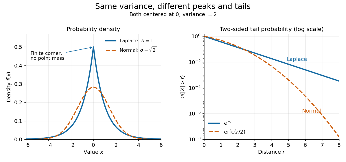
The figure compares a Laplace distribution with $\mu =0$, $b=1$ against a normal distribution with mean zero and standard deviation $\sigma =\sqrt{2}$: both have variance 2. The right panel uses a logarithmic scale for the two-sided tail probability $\mathbb{P}(|X|>r)$. Its straight Laplace distribution curve comes from $e^{-r}$; the normal distribution tail falls faster. Thus values far from the center can be more plausible under a Laplace distribution even after matching the variance. These are theoretical curves, not measured frequencies. The tails still have exponential decay; this is not a heavy-tailed distribution in the convention requiring every positive exponential moment to diverge.

Integrating either half of the probability density function gives the cumulative distribution functionIn particular $F(\mu )=1/2$. The basic moments areThus the scale is the expected value of the absolute distance from the center, and is not the standard deviation. ^[ref] A short way to obtain the moments is to note that $R=|X-\mu |$ has an exponential distribution with rate $1/b$: $\mathbb{P}(R>r)=e^{-r/b}$ for $r\ge 0$. Integrating gives $\mathbb{E}R=b$ and $\mathbb{E}{R}^2=2b^2$; the symmetric distribution gives the centered first moment zero.

The exponential distribution with rate $c>0$ has densityIt is the gamma distribution with shape one.

The gamma distribution with shape $a>0$ and rate $r>0$ has density