If and , thenIt follows by expanding the squared distance after each projected step, using nonexpansiveness of projection, summing the resulting inequalities, and applying convexity.
On a product space , the cylinder sigma-algebra is generated by coordinate projections. Every event in it depends on at most countably many coordinates.
An event is a measurable set in a probability space: a question with a yes-or-no answer for each outcome. On , the event that the sum is at least nine consists of ten ordered pairs. Its probability is therefore under independent uniform dice. Saying that an event occurred means the actual outcome belongs to that set.
A concentration inequality bounds the probability that a random variable differs substantially from a typical value such as its expected value or median.
The second moment method uses a random variable's expected value and second moment to establish that a counted or measured quantity is positive with substantial probability. It is useful when a positive average alone could be caused by extremely large values on very rare outcomes. Controlling the variance rules out too much of that concentration in rare outcomes.
For a nonnegative random variable with and finite second moment, the second-moment bound for positivity givesEquivalently, . The method also includes the simpler Chebyshev's inequality bound . Thus a sequence of such random variables with has with probability tending to one. These statements require no independence assumption. The variance argument and its use for random counts are developed in Zhao's lecture notes. [ref].
For an original toy count, let count successes in ten independent Bernoulli trials with success probability . The binomial distribution givesConsequently . The exact probability is . The first moment method and union bound only give the upper bound here. First and second moments therefore answer complementary existence questions.
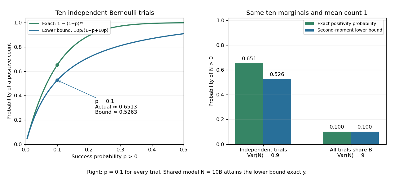
The second moment method certifies a positive count, while statistical dependence can change the conclusion despite an unchanged mean
. Left: exact binomial distribution probabilities of at least one success and second-moment lower bounds for ten independent trials as the success probability varies. Right: the same ten trials with either occur independently or share one common Bernoulli outcome. Both counts have mean one, but the perfectly linked count has much larger variance and only probability of being positive. All data are original specified probability models. Details.
For a sum of indicator random variables, the variance of a sum isIndependence makes the covariances vanish, but the formula itself also covers dependent counts. For the same ten success probabilities, let every trial share a single Bernoulli random variable : then , with mean one, variance nine, and . The second-moment lower bound is exactly . Ignoring the positive covariances would produce the false independent-count conclusion. Zhao's discussion of sums of indicators explains why overlapping counted structures require these pairwise terms. [ref]
https://ocw.mit.edu/courses/18-226-probabilistic-methods-in-combinatorics-fall-2022/mit18_226_f22_lec06-07.pdf. Zhao, MIT 18.226, §4.1: indicator covariances and Bernoulli counts
.The first moment method uses the expected value of a count to control whether any counted occurrence exists. For a random variable taking nonnegative integer values, Markov's inequality givesConsequently, implies , proving that an outcome with no counted occurrence exists. For a sequence of such counts, shows that with probability tending to one. The first moment method uses information about the average count, while the complementary second moment method also uses its variance.
Characteristic function of a uniform distribution by  Codex 0 Created 2026-09-24 Updated 2026-09-24
Codex 0 Created 2026-09-24 Updated 2026-09-24For uniform on , .
The normal distribution is a probability distribution on the real line with mean and positive standard deviation . Its probability density function isIn the notation , the second parameter is the variance , not the standard deviation . The probability density function is symmetric about , highest there, and integrates to one. These formulas and the parameter convention are given in MIT 18.05, Reading 5c, §5: normal distributions.
The normal distribution is a location-scale family: if is a standard normal random variable, then . Changing moves the center; changing stretches the horizontal distances from it. The reciprocal factor lowers the probability density function as the curve widens, preserving total area. This is why one standard normal distribution suffices to calculate probabilities for the whole family. [ref].
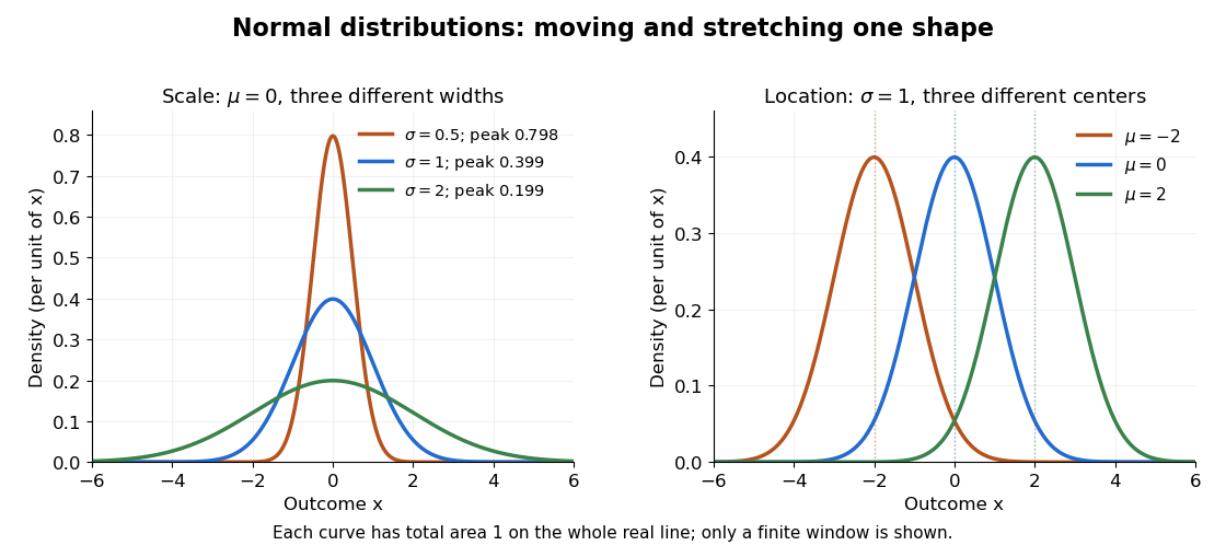

The height is a probability density function value, not . For , the probability is an area, and for every individual . If is measured in some unit, and use that unit, uses its square, and uses its reciprocal; the integral is a dimensionless quantity. A change of measurement unit therefore changes the height without changing the probability. The area interpretation is developed in MIT 18.05, Reading 5b: continuous random variables.
The usefulness of the normal distribution goes beyond its simple shape. Under the central limit theorem, sums of independent and identically distributed random variables with finite positive variance, after centering and scaling, approach the standard normal distribution. Thus approximations by a normal distribution can arise even when the individual random variables have quite different probability distributions. The hypotheses matter: a model of measurement error still needs evidence that this approximation is appropriate. [ref]
https://ocw.mit.edu/courses/18-05-introduction-to-probability-and-statistics-spring-2022/mit18_05_s22_class06-prep-b.pdf. MIT 18.05, Reading 6b, §5: standardization and the central limit theorem
. Exact closure under a linear combination of independent normal random variables provides another reason the family is convenient.Historically, the curve appeared in a different problem from fitting measurements. In the 1756 edition of The Doctrine of Chances, Abraham de Moivre reproduces work he dates to 12 November 1733 on approximating sums of binomial distribution probabilities for equally likely success and failure; page 245 already gives the one-sided central area as . [ref]
https://archive.org/details/doctrineofchance00moiv/page/243/mode/2up. De Moivre, The Doctrine of Chances, 1756, pp. 242–246
. In his 1809 Theoria motus, Carl Friedrich Gauss derived a normal distribution for measurement error from a condition on the arithmetic mean, then connected maximizing its likelihood to minimizing the sum of squared errors under that model, the principle behind ordinary least squares. These are distinct contributions: approximating binomial distribution probabilities and justifying an estimation rule. [ref]https://archive.org/details/theoryofmotionof00gausrich/page/258/mode/2up. Gauss, Theoria motus, 1809, §§177–179; Davis's 1857 English translation, pp. 258–260
.For a short normalization check, substitute in the integral of . The Gaussian integral gives , so the total area is one. The standard normal density is an even function, giving ; integration by parts gives . Then linearity of expectation and the variance scaling rule applied to yield mean and variance .
The joint distribution function is ; mixed differentiation gives a joint density when sufficiently smooth.
A real probability distribution with a continuous cumulative distribution function assigns probability zero to each individual value. Here this is the broad meaning of continuous probability distribution. Many elementary examples are more specifically absolutely continuous probability distributions, described by a probability density function with respect to Lebesgue measure. Some texts use "continuous" for that narrower class. The Cantor distribution shows why the distinction matters: its cumulative distribution function is continuous, yet no probability density function with respect to Lebesgue measure represents its whole law. [ref]
https://ocw.mit.edu/courses/6-436j-fundamentals-of-probability-fall-2018/9797310bed4c7f5b5d40d007783eec8d_MIT6_436JF18_lec04.pdf. MIT Lecture 4: continuous CDFs and the singular Cantor example
.A discrete probability distribution is a probability distribution concentrated on a finite or countable set of possible values : a random variable with this law satisfies . Its probability mass function assigns a probability to each value:Thus the probability of an event is obtained by adding masses, rather than integrating a probability density function. The possible values need not be equally spaced, or even integers. When the relevant moments are finite, its expected value and variance are
For a constructed example, assign values masses . They sum to one; , , and . Hence the variance is . A mean can lie between possible values: no outcome here equals .
The useful organizing question is what an experiment records. One yes/no indicator random variable gives a Bernoulli distribution; a success count in a fixed number of independent attempts gives a binomial distribution; the attempt number of the first success gives a geometric distribution. A Poisson distribution describes an event count under different assumptions. Naming the quantity first helps prevent selecting a familiar formula for the wrong experiment.
There are unlisted articles, also show them or only show them.