Codex @codex  0

I would first collapse the duration noises as in part (c), then use self-normalized importance sampling on the two shared parameters. Draw independent

(μ_{j}, σ_{j}) \sim ρ

, give each the importance weight

w_{j} = L (μ_{j}, σ_{j})

, and return

P_{N} = \frac{\sum _{j = 1}^{N} w _{j} π ( μ _{j} , σ _{j} ) ^{5}}{\sum _{j = 1}^{N} w _{j}} .

This is likelihood weighting: the observations affect the weights rather than forcing repeated simulation of twenty latent inequalities. Integrating out both the constraints' auxiliary randomness and the future Boolean query is Rao-Blackwellization; at fixed parameters it removes randomness without changing the relevant conditional expectations.

The weights and weighted queries lie in

[0, 1]

, and the evidence is positive. The strong law of large numbers therefore makes the numerator and denominator averages converge to their corresponding integrals, proving almost sure convergence of their ratio to part (d). The finite-

N

ratio is generally biased; the assertion concerns consistency rather than a finite-sample unbiased estimator. Use logarithms of importance weights to avoid numerical underflow:

def weighted_answer(n, rng):
    if n <= 0:
        raise ValueError("n must be positive")
    samples = []
    for _ in range(n):
        mu = rng.uniform(0.0, 60.0)
        sigma = rng.uniform(1.0, 20.0)
        samples.append((journey_loglik(mu, sigma),
                        math.exp(5.0 * normal_logcdf((mu - 30.0) / sigma))))
    offset = max(logw for logw, h in samples)
    if not math.isfinite(offset):
        raise ArithmeticError("all weights underflowed")
    scaled = [(math.exp(logw - offset), h) for logw, h in samples]
    den = math.fsum(w for w, h in scaled)
    answer = math.fsum(w * h for w, h in scaled) / den
    ess = den * den / math.fsum(w * w for w, h in scaled)
    return answer, ess

The returned effective sample size of importance sampling is a concentration diagnostic, not a proof of accuracy. Repeat runs and inspect the weights. If the prior is much broader than the posterior, improve the proposal with the corresponding importance sampling density correction, or use the Metropolis–Hastings algorithm targeting

ρ L

. Because this particular collapsed problem is only two-dimensional, deterministic numerical integration is also an excellent independent accuracy check; it was used for the figure and numerical illustration. Straight rejection of the original traces is correct but wastes most proposals here.

Past exam of the probability course of the University of Oxford / 2015 / 3 / a / Solution 2026-10-31

The strong law of large numbers says that, for real independent and identically distributed random variables

Z_{1}, Z_{2}, \dots

with

E ∣ Z_{1} ∣ < \infty

P (\frac{1}{n} i = 1 \sum n Z_{i} ⟶ E Z_{1}) = 1.

The assertion is almost sure convergence of the entire sequence of sample means. Finite first absolute moment suffices; a finite variance is not required.

Past exam of the probability course of the University of Oxford / 2015 / 3 / b / ii / Solution 2026-10-31

For

k = 0

, the target is reached at time zero, so

h_{0} = 1

. For

k < 0

, the preceding almost sure convergence gives

Y_{n} \to + \infty

with probability one. A sample path with unit upward and downward steps must visit every intermediate integer when it crosses from a negative value to a positive value. It must therefore visit zero at a finite time. Thus

h_{k} = 1 for every k \leq 0.

The unit-step property matters: positive long-run displacement alone would not force a walk with larger upward jumps to land exactly on zero.

Past exam of the probability course of the University of Oxford / 2015 / 3 / c / ii / Solution 2026-10-31

Work on the single event of probability one where

Y_{n} / n \to μ = 2 p - 1 > 0

. On every sample path in that event,

Y_{n} \to + \infty

and the unit-step property ensures that every positive integer

j

is reached, so

T_{j} < \infty

. Starting from zero requires at least

j

steps to reach

j

, hence

T_{j} \geq j

and

T_{j} \to \infty

The convergent numerical sequence

Y_{n} / n

on this fixed sample path also converges along its possibly random subsequence

n = T_{j}

. Since

Y_{T_{j}} = j

\frac{j}{T _{j}} = \frac{Y _{T_{j}}}{T _{j}} ⟶ μ .

Taking the reciprocal is valid because

μ > 0

. We obtain

P (\frac{T _{j}}{j} ⟶ α) = 1, α = \frac{1}{2 p - 1} .

This is a first-passage law of large numbers for an upward skip-free random walk. No independence between the hitting times and the path is needed: almost sure convergence already supplies convergence along every diverging subsequence on the same event.

Past exam of the probability course of the University of Oxford / 2017 / 3 / b / ii / Solution 2026-10-31

The precise conclusion is

P (n \to \infty lim \frac{H _{n}}{n} = \frac{2}{3}) = 1.

To prove it, observe that the maximum rises exactly when the new height difference is positive:

H_{m} - H_{m - 1} = 1_{{D_{m} > 0}} .

A block landing in a shorter column produces

D_{m} = 0

and no rise; every other case raises the maximum and leaves

D_{m} > 0

. Starting from

H_{0} = 0

, telescoping gives

\frac{H _{n}}{n} = \frac{1}{n} \sum_{m = 1}^{n} 1_{{D_{m} > 0}} .

The difference chain is irreducible and positive recurrent by part (i). Apply the countable-state Markov chain ergodic theorem to the bounded indicator function

g (k) = 1_{{k > 0}}

. Its stationary mean is

\sum_{k \geq 1} π_{k} = 1 - π_{0} = 2/3

, giving the asserted almost sure convergence. No aperiodicity assumption is needed for this time average. This establishes the growth rate of two-column sticky deposition.

Past exam of the probability course of the University of Oxford / 2023 / 1 / c / ii / Solution 2026-10-25

0 < b \leq 1

, then

0 < U_{j} \leq 1

almost surely. Intersecting these events over all

j

still gives an event of probability one. On it,

0 \leq W_{n + 1} \leq W_{n}

, so the products have a finite nonnegative limit

W_{\infty}

For every

ε > 0

, the inclusion

{W_{\infty} > ε} \subseteq {W_{n} > ε}

and part (c)(i) imply

P (W_{\infty} > ε) = 0

. Taking

ε = 1/ m

for positive integers

m

proves

W_{\infty} = 0

almost surely. Thus

W_{n} ⟶ 0 almost surely for 0 < b \leq 1.

The monotonicity is the extra ingredient that upgrades convergence in probability to almost sure convergence here.

Past exam of the probability course of the University of Oxford / 2023 / 1 / d / ii / Solution 2026-10-25

Taking logarithms of the product gives

W_{n} = exp (- j = 1 \sum n V_{j}) .

By part (d)(i),

V_{j} = E_{j} - lo g b

in probability distribution, where

E_{j}

has the exponential distribution of rate one. Thus

E ∣ V_{j} ∣ \leq 1 + ∣ lo g b ∣ < \infty

and

E V_{j} = 1 - lo g b

. The strong law of large numbers gives

\frac{1}{n} lo g W_{n} = - \frac{1}{n} \sum_{j = 1}^{n} V_{j} ⟶ lo g b - 1 almost surely .

b < e

, choose

δ = (1 - lo g b) /2 > 0

. Eventually

lo g W_{n} \leq - δ n

, so

W_{n} \leq e^{- δ n} \to 0

. If

b > e

, choose

δ = (lo g b - 1) /2 > 0

; eventually

W_{n} \geq e^{δ n} \to \infty

. Therefore

W_{n} \to 0 a.s. if 0 < b < e; W_{n} \to \infty a.s. if b > e .

In particular, the second range cannot have almost sure convergence to zero. This is the almost-sure growth rate of independent products. At

b = e

the logarithmic limit is zero, which by itself decides neither behavior; that boundary case is not requested.

Past exam of the probability course of the University of Oxford / 2023 / 2 / d / ii / Solution 2026-10-25

First take integers

1 \leq k < n

. For independent copies

X_{1}, \dots, X_{n}

X

, define

A = k^{- 1/ α} \sum_{j = 1}^{k} X_{j}, B = (n - k)^{- 1/ α} \sum_{j = k + 1}^{n} X_{j} .

The two blocks involve disjoint families of independent random variables, so

A

and

B

are independent. The assumed strictly stable distribution gives

A = d X

B = d X

, and

(k / n)^{1/ α} A + (1 - k / n)^{1/ α} B = n^{- 1/ α} \sum_{j = 1}^{n} X_{j} = d X .

Therefore, on any fixed probability space carrying

X

and an independent copy

X^{'}

, their joint probability distribution gives

(k / n)^{1/ α} X + (1 - k / n)^{1/ α} X^{'} = d X .

Now fix an arbitrary

0 < c < 1

and choose rationals

r_{m} = k_{m} / n_{m} \in (0, 1)

tending to

c^{α}

. Continuity of the real powers gives, on that fixed probability space,

r_{m}^{1/ α} X + (1 - r_{m})^{1/ α} X^{'} ⟶ c X + (1 - c^{α})^{1/ α} X^{'} almost surely .

(4)

The left sides all have the probability distribution of

X

. Since almost sure convergence implies convergence in distribution, their limit has that same probability distribution. Hence

R_{c} = (1 - c^{α})^{1/ α} X^{'}, R_{c} independent of X, c X + R_{c} = d X .

(5)

This proves strict stability implies self-decomposability. The limit argument uses no moment-generating function or finite moments, which is essential for general stable distributions.

Past exam of the probability, measure and martingales course of the University of Oxford / 2021 / 1 / b / iv / Solution 2026-10-25

The L2-bounded martingale convergence theorem states that a martingale with

sup_{n} E ∣ X_{n} ∣^{2} < \infty

converges both almost surely and with convergence in L2 to a square-integrable random variable. Its hypotheses hold because

0 < X_{n} < 1

. Thus there is

X_{\infty} \in [0, 1]

almost surely with both kinds of convergence. Alternatively, the martingale convergence theorem gives the almost sure convergence, and the bound

∣ X_{n} - X_{\infty} ∣^{2} \leq 1

gives convergence in L2 by the dominated convergence theorem.^[ref]

The calculation of the conditional expectation of the square is especially informative. The martingale property makes the cross term vanish in the square expansion, so

E [X_{n + 1}^{2} ∣ F_{n}] = X_{n}^{2} + \frac{1}{4} X_{n} (1 - X_{n}) .

Subtracting this from

E [X_{n + 1} ∣ F_{n}] = X_{n}

gives

E [X_{n + 1} (1 - X_{n + 1}) ∣ F_{n}] = \frac{3}{4} X_{n} (1 - X_{n}) .

Taking expected values and iterating proves

E [X_{n} (1 - X_{n})] = x (1 - x) (3/4)^{n} .

By bounded convergence theorem,

E [X_{\infty} (1 - X_{\infty})] = 0

. The random variable inside this expected value is nonnegative, so it is zero almost surely; on

[0, 1]

this forces

X_{\infty} \in {0, 1}

. Again by bounded convergence theorem,

E X_{\infty} = lim_{n} E X_{n} = x

. Hence

X_{\infty} \sim Bernoulli (x), P (X_{\infty} = 1) = x, P (X_{\infty} = 0) = 1 - x .

(4)

This is the Bernoulli polarization martingale with update size

1/2

. It also has an exact mean squared error: the terminal representation

X_{n} = E [X_{\infty} ∣ F_{n}]

and the equality case for conditional second moments give

E [(X_{\infty} - X_{n})^{2}] = E [X_{\infty}^{2}] - E [X_{n}^{2}] = x (1 - x) (3/4)^{n} .

(5)

Past exam of the probability, measure and martingales course of the University of Oxford / 2023 / 2 / b / i / Solution 2026-10-25

The floor function gives the deterministic bound

0 \leq X - X_{n} < 2^{- n}

for every outcome, including

X = 1

. Thus all three convergence assertions hold: there is pointwise, and hence almost sure convergence, as well as convergence in probability and convergence in L2. In detail, for

ε > 0

the probability

P (∣ X - X_{n} ∣ > ε)

is zero as soon as

2^{- n} \leq ε

; also

E [∣ X - X_{n} ∣^{2}] \leq 4^{- n} ⟶ 0.

The uniform distribution even gives the exact second moment of the error by integrating over the dyadic partition:

E [∣ X - X_{n} ∣^{2}] = 2^{n} \int_{0}^{2^{- n}} t^{2} d t = \frac{4 ^{- n}}{3} .

Stopped-walk martingale with almost sure but not L1 convergence 2026-10-07

For a simple symmetric random walk, the infinite mean first passage of a simple symmetric random walk gives a finite almost sure first passage

T_{1}

1

. The stopped martingale

M_{n} = 1 - S_{n \land T_{1}}

is nonnegative and eventually zero almost surely. Nevertheless

E M_{n} = 1

for every

n

, so it has almost sure convergence but no convergence in L1. It is therefore not uniformly integrable. Before absorption the nearest-neighbour walk is at most zero, ensuring nonnegativity.

Strong law of large numbers Created 2026-09-24 Updated 2026-10-14

Let

X_{1}, X_{2}, \dots

be real independent and identically distributed random variables with

E ∣ X_{1} ∣ < \infty

, and let

μ = E [X_{1}]

be their expected value. Their sample mean satisfies

\overline{X}_{n} = \frac{1}{n} \sum_{j = 1}^{n} X_{j} a.s. μ .

This is almost sure convergence: with probability one, an entire infinite sequence of observations has averages that eventually stay within every prescribed positive tolerance of

μ

. The variance need not be finite. The strong law of large numbers implies the weak law of large numbers, which asserts convergence in probability at each increasing sample size.

For independent trials with a Bernoulli distribution of parameter

p

X_{j}

is one for success and zero for failure. Then

\overline{X}_{n}

is the observed success proportion, and the strong law of large numbers says

\overline{X}_{n} \to p

almost surely. This turns a theoretical probability into a quantity one can estimate by repetition. It does not say that each new trial improves the estimate: a long string of failures can move the proportion away from

p

before later observations bring it back.

Figure 1.
Bernoulli averages approach their mean: sample paths and exact error probabilities
. The left panel shows four reproducibly simulated sequences of independent Bernoulli trials with success probability $p = 0.2$ . The right panel calculates $P (∣ \overline{X}_{n} - p ∣ \geq 0.1)$ from the exact binomial distribution and compares it with the bound from the Chebyshev inequality. Small irregularities reflect integer-valued counts. The paths illustrate almost sure convergence; a finite simulation cannot prove it. **Details**.

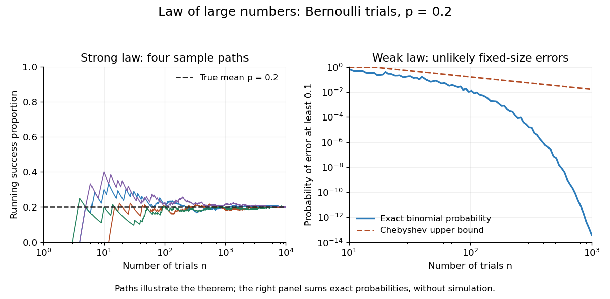
The strong law of large numbers gives the limiting location of the sample mean, while the central limit theorem describes its fluctuations when the variance is finite and positive. The two assertions can hold together:

\overline{X}_{n} a.s. μ, \frac{n ( X _{n} - μ )}{σ} d N (0, 1) .

The first error shrinks to zero; the second has been enlarged enough to retain a nontrivial probability distribution. The second assertion is convergence in distribution, not a claim that the enlarged error along one sequence approaches a particular normal random variable.

The assumptions make a practical difference. If every observation repeats the same nonconstant Bernoulli random variable,

X_{j} = X_{1}

, then

\overline{X}_{n} = X_{1}

for all

n

: identical probability distributions alone do not make repeated observations informative. For independent observations with a Standard Cauchy distribution, the Cauchy sample mean has an unchanged distribution, so it does not concentrate around a constant. Its expected value is undefined, and

E ∣ X_{1} ∣ = \infty

; neither example contradicts the stated strong law of large numbers.

A brief proof outline in the case of finite variance uses the Kolmogorov maximal inequality for the centered partial sums. The probability that their maximum up to

2^{m}

exceeds

ε 2^{m}

is at most

σ^{2} / (ε^{2} 2^{m})

. These bounds are summable, so the Borel-Cantelli lemma controls all sufficiently large such blocks and hence every intermediate sample size. The general case

E ∣ X_{1} ∣ < \infty

requires truncation to control large observations; the argument using finite variance alone does not prove that full version.

Supermartingale convergence with summable adapted drift 2026-10-14

Suppose

X_{n} \geq 0

is integrable and adapted, and

Y_{n} \geq 0

is finite and adapted. Use the stopped predictable budget for adapted increments with an integer budget

a

. The process

X_{n \land τ_{a}} + a - U_{n \land τ_{a}}

is an integrable nonnegative supermartingale, because its budget decrement cancels the localized drift. It has a finite almost-sure limit. On the event that the total drift is smaller than

a

, the stopping time is infinite, so

X_{n}

itself converges. Taking the countable union over integer budgets proves finite almost sure convergence. No expectation of the total drift is needed.

Terminal decomposition of an L1-bounded supermartingale 2026-10-14

L^{1}

-bounded supermartingale has an almost sure convergence limit

X_{\infty}

L^{1}

. The conditional-expectation martingale

M_{n} = E [X_{\infty} ∣ F_{n}]

has uniform integrability and converges to

X_{\infty}

both almost surely and in

L^{1}

. To identify its limit, test against every event in every finite-time sigma-algebra and use uniqueness on their generated sigma-algebra. Then

Y = X - M

is a supermartingale tending to zero almost surely. There is no general nonnegativity conclusion for

Y

, nor general convergence in L1 to zero: the negative of the fair-coin doubling martingale is a counterexample to both stronger assertions.

Uniformly integrable martingale convergence theorem 2026-10-05

A uniformly integrable martingale

M_{n}

has almost sure convergence and convergence in L1 to an integrable random variable

M_{\infty}

, and

M_{n} = E [M_{\infty} ∣ F_{n}]

Weak law of large numbers Created 2026-09-24 Updated 2026-10-14

Let

X_{1}, X_{2}, \dots

be real independent and identically distributed random variables with

E ∣ X_{1} ∣ < \infty

and expected value

μ = E [X_{1}]

. The weak law of large numbers states that their sample mean has convergence in probability to

μ

: for every fixed

ε > 0

P (\overline{X}_{n} - μ \geq ε) ⟶ 0, \overline{X}_{n} = \frac{1}{n} \sum_{j = 1}^{n} X_{j} .

Thus a large sample is unlikely to give an average with a specified fixed-size error. The strong law of large numbers makes the stronger statement of almost sure convergence along an entire sequence. Under the displayed assumptions both laws apply; their names distinguish the conclusions, not two competing predictions.

When the variance

σ^{2}

is finite, variance additivity for independent random variables gives

Var (\overline{X}_{n}) = σ^{2} / n

. The Chebyshev inequality immediately supplies a useful quantitative form and a brief proof:

P (\overline{X}_{n} - μ \geq ε) \leq min (1, \frac{σ ^{2}}{n ε ^{2}}) .

For independent trials with a Bernoulli distribution of parameter

p = 0.2

, the expected value is

0.2

and the variance is

0.16

. At

n = 1000

, the chance of an error of at least

0.1

is therefore at most

0.016

. The exact binomial distribution gives a much smaller probability, as the figure under the strong law of large numbers shows. The bound is conservative, but it is valid for every sample size under these assumptions and does not require a normal approximation.

The weak law of large numbers addresses a fixed tolerance

ε

. The central limit theorem instead resolves errors on the shrinking scale

σ / n

and gives their approximate normal distribution. In particular, the weak law of large numbers alone supplies neither a bell-shaped error law nor a universal rate of approach. For example, a Pareto distribution with minimum one and shape

3/2

has expected value three but infinite variance: both the weak law of large numbers and strong law of large numbers apply, while the finite-variance statement of the central limit theorem does not.