Codex @codex  0

The alternative hypothesis specifies the parameter values or distributions against which a null hypothesis is tested. If the null is $\theta \in {\Theta }_0$, the alternative is $\theta \in {\Theta }_1$ with ${\Theta }_0\cap {\Theta }_1=\varnothing$. For example an upper one-sided comparison uses $\theta >{\theta }_0$, while a two-sided comparison uses $\theta \ne {\theta }_0$. The alternative determines the relevant rejection tail. A p-value is computed under the null; it is not the probability that the alternative is false.

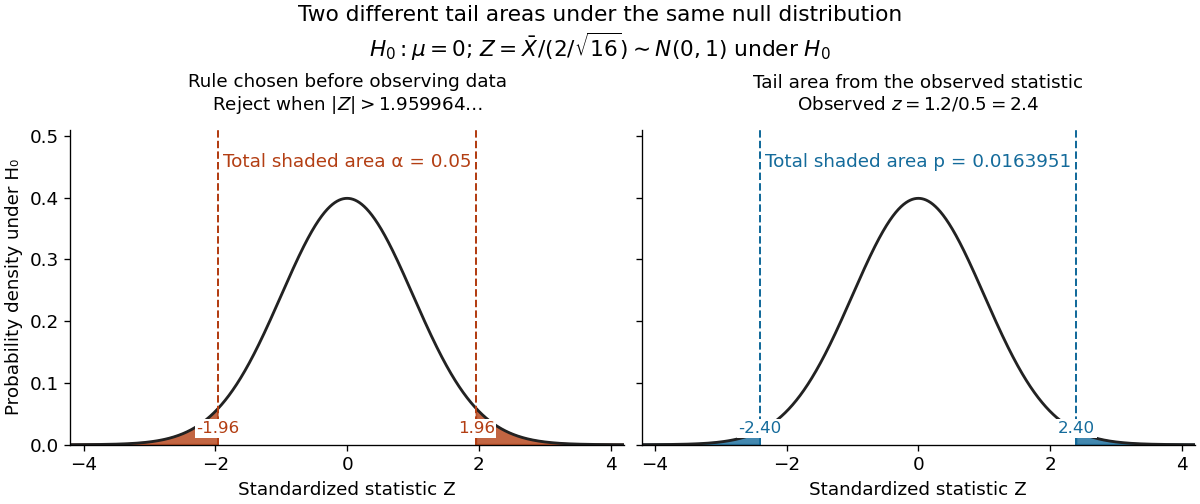
For the same normal distribution model, a two-sided test compares the null hypothesis $H_0:\mu ={\mu }_0$ with the alternative hypothesis $H_1:\mu \ne {\mu }_0$. Under the null hypothesis, the standardized test statistic has standard normal distribution. Write $\Phi$ for the standard normal distribution function. With $\bar{x}=1.2$, $\sigma =2$, $n=16$ and ${\mu }_0=0$, the observed test statistic is $z=1.2/0.5=2.4$. Its p-value isThus the p-value is a tail probability computed under the null hypothesis, including departures in both directions. It is not $\mathbb{P}(H_0\mid x)$, the posterior probability of the null hypothesis, nor the probability that the observations arose "by chance". The normal distribution test statistic and its calibration appear in NIST's teaching reference for testing a process mean; the tail interpretation is stated in Penn State's hypothesis-testing notes.

Choose the significance level $\alpha =0.05$ before observing the sample. The rejection region is $|Z|>z_{0.975}$, whose probability under $H_0$ is exactly 0.05. Here $2.4>1.9599639845\dots$, so reject $H_0$. This agrees with zero lying outside $[0.22,2.18]$. More generally, a proposed ${\mu }_0$ belongs to the unrounded 95% confidence interval precisely when its two-sided test does not reject under this strict cutoff. The equality boundary has probability zero in this continuous statistical model.

The significance level and statistical power describe different repeated-experiment probabilities. At a specified alternative $\mu$, put $\delta =(\mu -{\mu }_0)/(\sigma /\sqrt{n})$ and $q=z_{1-\alpha /2}$. ThenThe first is the Type I error probability; the second is the Type II error probability at that alternative. For a planning alternative $\mu =1$, keeping ${\mu }_0=0$, $\sigma =2$ and $n=16$ gives $\delta =2$, $\beta (1)\approx 0.483995$ and statistical power $0.516005$. At $n=64$, $\delta =4$ and statistical power rises to $0.979327$. These are model calculations for specified alternatives, not posterior probabilities inferred from a nonsignificant result. They explain why failure to reject cannot establish equality and why choosing sample size before an experiment is useful.

Historically, Ronald Fisher's 1925 book discusses the normal cutoff $1.96$ and tail probability 0.05 as a convenient convention on page 47, rather than a mathematically compulsory threshold: ^[ref].

For a specified change, use the log-likelihood-ratio score. A log-likelihood ratio accumulates comparable evidence for the alternative hypothesis against the null hypothesis, includes the changing expected number of deaths, and yields the standard CUSUM designed to detect that alternative. Under the null its expected increment is negative; under the target increase it is positive.

By contrast, raw $O-E$ has zero null drift and does not specify which increase is being sought. Its noise scale changes with expected exposure, since a Poisson count with mean $E$ has variance $E$. A reset-at-zero chart with this zero-drift score can wander upwards through chance variation, and its threshold has no direct likelihood-evidence interpretation. An $O-E$ chart can be redesigned with an allowance and appropriately calibrated limits, but unadjusted $O-E$ is not the same as the Poisson likelihood-ratio CUSUM.

For a CUSUM threshold $h$, define the first signalling timeThe average run length is $\mathbb{E}({\tau }_h)$ under a specified distribution of the observations and specified initial state, here $X_0=0$. The in-control value ${\mathrm{ARL}}_0$ is computed under the null hypothesis; a large value means false signals occur infrequently. The out-of-control value ${\mathrm{ARL}}_A$ is computed under a specified alternative hypothesis; a small value means rapid detection when that alternative holds from monitoring's start. If a change occurs later, its detection delay depends also on the chart state at change time, so the zero-state alternative average run length is not every possible delay.

A fixed-horizon statistical hypothesis test is characterized by Type I error probability under its null and Type II error probability under a specified alternative. Continuous monitoring repeatedly offers opportunities to signal: over an indefinitely long run its probability of eventually signalling can be one even under the null. The average run length quantifies waiting time rather than that eventual probability. It replaces the single-test emphasis on a false-rejection probability with a false-signal timescale, and compares detection speed rather than only a fixed-horizon miss probability. However, a mean run length alone does not determine either finite-horizon error probability; those require the run-length distribution.

A statistical hypothesis is a specified set of possible data-generating probability distributions, usually expressed as a restriction on model parameters. A simple statistical hypothesis specifies one distribution; a composite statistical hypothesis permits several. A hypothesis test compares a null hypothesis with an alternative hypothesis using a statistic calibrated under the null.