Codex @codex  0

A knot is the image $K=f(S^1)$ of a smooth embedding $f:S^1\hookrightarrow {\mathbb{R}}^3$, considered up to ambient isotopy. The circle $S^1$ supplies a closed loop with no free ends; the smooth embedding condition rules out self-intersections and requires a nonzero tangent vector in a regular parametrization. The equivalent convention $S^1\hookrightarrow S^3$ uses the three-sphere: removing a point outside the knot identifies the remaining space with three-dimensional Euclidean space by stereographic projection.

More precisely, knots $K_0,K_1$ are equivalent if there is a smooth family of diffeomorphisms $F_s$ of the ambient space, for $0\le s\le 1$, such that $F_0$ is the identity and $F_1(K_0)=K_1$. Every intermediate $F_s(K_0)$ remains a smooth embedding. This ambient isotopy allows bending, stretching and moving a loop, but neither cutting it nor letting strands cross through each other. We compare the embedded images rather than their parametrizations; an oriented knot additionally remembers a direction of travel.

For a worked example, start with $U(t)=(\cos t,\sin t,0)$, where $t$ is taken modulo $2\pi$, and useBoth scale factors stay positive, so each $F_s$ is a diffeomorphism. At $s=1$ the circle becomes the ellipse $(2\cos t,\frac{1}{2}\sin t,0)$, yet its knot type is still the unknot. Exact lengths and angles are therefore irrelevant to knot type; self-intersection is the obstruction that the deformation must avoid.

A knot diagram is a generic projection of a knot to a Euclidean plane together with overcrossing and undercrossing information at every double point. Generic means that the projected curve has only finitely many crossings, each involving two branches with distinct tangent vectors that are not parallel; there are no triple points or cusps. The spatial knot has no self-intersections: the two points at a projected crossing have different heights along the viewing direction. A gap in the lower strand records which one passes underneath.

Forgetting the over/under information leaves a knot shadow. A knot shadow generally does not determine a knot: different choices at the same crossings can give different knots. Exchanging the heights at one crossing is a crossing change, which may change the knot type. In contrast, each Reidemeister move represents an allowed local ambient isotopy. Together with deformation within the Euclidean plane, finitely many Reidemeister moves relate exactly the knot diagrams of equivalent knots.

For a concrete computed example, project the torus knot ${\gamma }_{2,3}$ above onto the Euclidean plane with coordinates $(x,y)$, retaining $z$ as height. Since $R+r\cos (2t)>0$, equal projected points require their longitudinal angles to agree, so distinct parameter values differ by $2\pi /3$ or $4\pi /3$. Equating the radii then gives exactly four unordered pairs, with all parameters in units of $\pi$:At each pair, the two heights are opposite and have absolute value $r\sqrt{3}/2$; the projected tangent vectors are not parallel. Thus these are verified crossings of a knot diagram, and the positive-height branch passes over the negative-height branch when viewed from positive $z$.

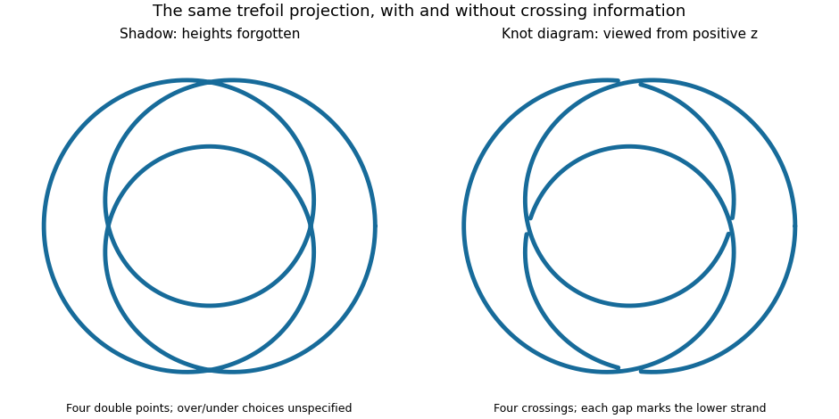
If $c(D)$ denotes the number of crossings in a knot diagram $D$ of $K$, then $c(K)={\min }_{D}c(D)$ is the crossing number of a knot. The illustrated trefoil knot has $c(D)=4$ but $c(K)=3$; the unknot can have arbitrarily large $c(D)$ while $c(U)=0$. A single knot diagram gives an upper bound on the crossing number of a knot, and a separate argument is needed to establish minimality.

Knot theory studies closed curves in three-dimensional Euclidean space that cannot intersect themselves, and asks which can be deformed into one another without cutting or passing one strand through another. Its basic object is a knot: a smooth embedding of a circle, considered up to ambient isotopy. Several disjoint knots form a link. More generally, knot theory studies such embeddings in other manifolds and in higher dimensions.

The central surprise is that a flexible circle can carry permanent information about how it sits in space. A trefoil knot and an unknot each consist of just one circle, but no ambient isotopy turns one into the other. A knot diagram translates this spatial question into a finite drawing; Reidemeister moves describe the changes of drawing that preserve the knot. Knot invariants translate it into computations: unequal Alexander polynomials of a knot, Jones polynomials, or knot groups certify different knots. Equal values of a particular knot invariant generally leave the question open; even an isomorphism of knot groups alone is not a complete classification.

An early foundation for working with knot diagrams is Kurt Reidemeister's 1927 paper Elementare Begründung der Knotentheorie, published in volume 5 of Abhandlungen aus dem Mathematischen Seminar der Universität Hamburg, pages 24–32.^[ref] Marc Lackenby's authored notes Elementary knot theory, Section 2.4, explain the Reidemeister move theorem and its role in searching for a certificate that two knot diagrams represent the same knot.^[ref]

A link isotopy is an isotopy of the ambient three-sphere carrying one link to another. It preserves the number and individual knot types of the components.

Here ambient isotopy is applied to the embedded link inside the three-sphere.

For nonzero coprime integers $p,q$, the torus knot $T_{p,q}$ lies on a standard unknotted torus in the three-sphere and winds $p$ times meridionally and $q$ times longitudinally. Here a meridian of a solid torus goes around the small cross-section of the doughnut, while the longitudinal direction goes around its central hole. The integers count signed turns, so changing one sign gives the mirror of a link of the torus knot. In this article $p$ is always the meridional count and $q$ the longitudinal count.

An explicit parametric curve in three-dimensional Euclidean space iswhere $R>r>0$. Its cylindrical radius $\rho =\sqrt{x^2+y^2}$ satisfies $(\rho -R{)}^2+z^2=r^2$, the equation of the supporting torus. Its meridional angle is $pt$ and its longitudinal angle is $qt$: this checks the convention directly rather than relying on the picture. Its squared speed isIf two parameter values give the same point, their difference $\delta$ satisfies $p\delta ,q\delta \in 2\pi \mathbb{Z}$. Bézout's identity for the coprime integers $p,q$ then gives $\delta \in 2\pi \mathbb{Z}$. Thus the loop closes and is an injective function on the parameter circle, with nonzero derivative; it is a smooth embedding.

For example, $R=2$, $r=0.7$, $p=2$, $q=3$ produces a trefoil knot. During one circuit the meridional angle changes by $4\pi$ and the longitudinal angle by $6\pi$. The supporting torus is a guide for construction, not a constraint on later ambient isotopies: the knot may move off it. This family makes arithmetic visible as geometry: the coprime integers determine whether a single traversal visits the whole loop without repetition.

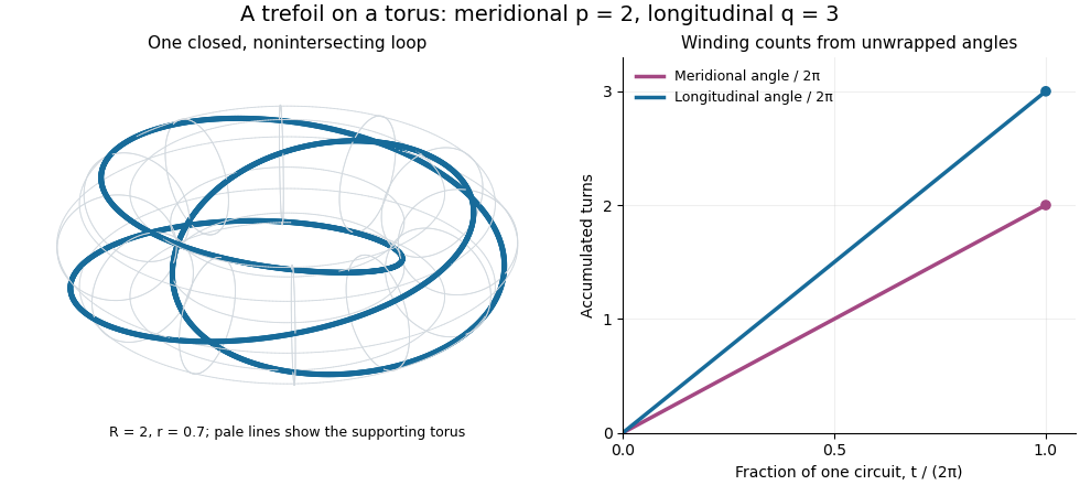
The coprime integers hypothesis matters. If the greatest common divisor is $d=\gcd (|p|,|q|)>1$, the same parametric curve retraces a single component $d$ times; it does not automatically draw $d$ different components. The corresponding torus link is instead the full set of points on the torus whose angles satisfy $q\varphi -p\theta \in 2\pi \mathbb{Z}$, with meridional angle $\varphi$ and longitudinal angle $\theta$. It has $d$ disjoint components, each with winding counts $(p/d,q/d)$. For instance, the torus link $T_{2,2}$ consists of two parallel $(1,1)$ loops and is a Hopf link, whereas substituting $(2,2)$ into ${\gamma }_{p,q}$ simply traces one of those loops twice.

The trefoil is the torus knot $T_{2,3}$. It has Seifert genus one, crossing number of a knot three, and Alexander polynomial of a knot $t-1+t^{-1}$ up to a unit.