Attosecond physics

Attosecond physics resolves changes on the scale of $10^{-18}$ seconds, especially Electron dynamics. Its central trick is to convert a short optical event into an experimentally accessible energy or phase change. A broad optical spectrum provides the ingredients for a short optical pulse; their spectral phases determine when those ingredients add constructively. High harmonic generation supplies the optical spectrum, while RABBITT and attosecond streaking supply complementary timing measurements. XUV denotes extreme ultraviolet radiation.

There are two separate timing problems: characterize the incident optical pulse, then infer the response of the target. A photoelectron measurement mixes the incident spectral phase, the target's transition response and the probing electric field. Recovering one requires constraints on the others. These methods measure distributions of photoelectron energies over repeated shots, rather than photographing a moving atomic orbital.

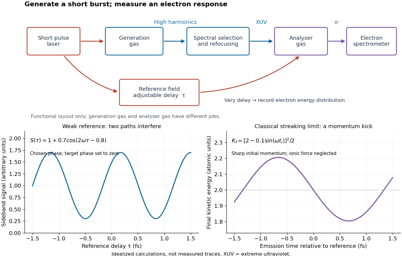
High harmonic generation converts an intense driving electric field into radiation at high integer multiples of its frequency. High harmonic generation in a gas is a process in nonlinear optics: an Electron can leave a neutral target by tunnel ionization, gain kinetic energy in the driving electric field, and return to radiate upon recombination. This three-step picture is an approximate account of a probability amplitude for emission in quantum mechanics, not a measured path of one Electron.^[ref]

Why odd multiples? In an ideal centrosymmetric gas driven by a single frequency, assume the radiating electric dipole moment satisfies $d(t+T/2)=-d(t)$, where $T$ is the driving period. Its Fourier series coefficient obeys $d_q=-(-1{)}^q{d}_q$, so every even coefficient vanishes. A finite envelope, an oriented target or an additional driving frequency can invalidate that symmetry argument. Producing many odd components also does not prove that their spectral phases form a short optical pulse.

The 1988 report involving Anne L'Huillier observed odd multiples of a $1064\mathrm{nm}$ driving wavelength in rare gases, reaching order 33 in argon. The unexpectedly slow fall of yield beyond the fifth order supplied a broad spectral plateau. A spectral observation alone did not establish the relative spectral phases needed for an attosecond pulse train.^[ref]

For an original classical calculation of the return step, neglect the residual ion's Coulomb force after release. Take a spatially uniform driving electric field $E(t)=E_0\cos \omega t$, an Electron of electric charge $-e$ and mass $m$, and zero initial position and velocity at $t_i$. With $\alpha =\omega t_i$ and $\beta =\omega t$, integrating Newton's second law givesA return requires $\beta >\alpha$ and $x(t)=0$. Define the cycle-averaged free-electron quiver kinetic energySearching the first-return solutions for release phases $0<\alpha <\pi /2$ gives a maximum near $\alpha =0.3134$ and $\beta =4.3990$, with $K_{\mathrm{return}}\simeq 3.1731U_p$. For a chosen ionization energy $I_p$, recombination into the initial state can therefore emit a photon with energy up to approximately $I_p+3.17U_p$ in this model. This is an upper return-energy scale, not a prediction of the emitted yield. It omits release probabilities, quantum interference, propagation, phase matching and depletion of the neutral gas.

The calculation explains why a long driving wavelength can increase the available return energy: at fixed $E_0$, $U_p$ grows as ${\omega }^{-2}$. It does not say that conversion efficiency improves. The Electron must return with a probability amplitude for emission that survives the microscopic dynamics and adds coherently across the gas.

An attosecond pulse train contains repeated short optical pulses. For a group of odd multiples of a common driving frequency, the separation is half the driving period when the relative spectral phases recur. The construction resembles mode locking, but the participating components come from high harmonic generation, rather than separate resonant modes of a laser oscillator.

Choose $N$ equal-amplitude, monochromatic odd components with orders $q_j=q_0+2j$, $j=0,\dots ,N-1$, and odd $q_0$. Fix the complex-field conventionHere $I$ is a normalized light intensity after averaging the fast carrier oscillations. Setting every ${\varphi }_j=0$ and summing a geometric series givesAt the removable singularities take the continuous limit. Maxima repeat every $T/2=\pi /\omega$; the first zeros on either side of a maximum lie at $t=\pm T/(2N)$. The zero-to-zero width is $T/N$, which is not the full width at half maximum.

Choose orders $13,15,17,19,21$ and driving wavelength $\lambda =800\mathrm{nm}$. Using $T=\lambda /c$ with the speed of light $c$ gives $T=2.66851\mathrm{fs}$ and burst spacing $1.33426\mathrm{fs}$. Solving the exact half-maximum equation gives a full width at half maximum of approximately $240.6$ attoseconds. These are values of the specified five-component model, not measurements from the 2001 experiment.

A deliberately chosen spectral phase ${\varphi }_q=q\omega t_0$ translates the whole attosecond pulse train by $t_0$ without changing its shape. Adding $\kappa (q-17{)}^2/2$ makes neighboring phase increments unequal: the same component intensities then produce a different temporal profile. For the choice $t_0=0.20\mathrm{fs}$ and $\kappa =0.08$ radians per squared harmonic order, the adjacent-component delay estimates arenamely $0.0981$, $0.1660$, $0.2340$ and $0.3019\mathrm{fs}$ for $q=13,15,17,19$. This finite difference estimates the group delay at the pair's midpoint. It is not a single common arrival time.

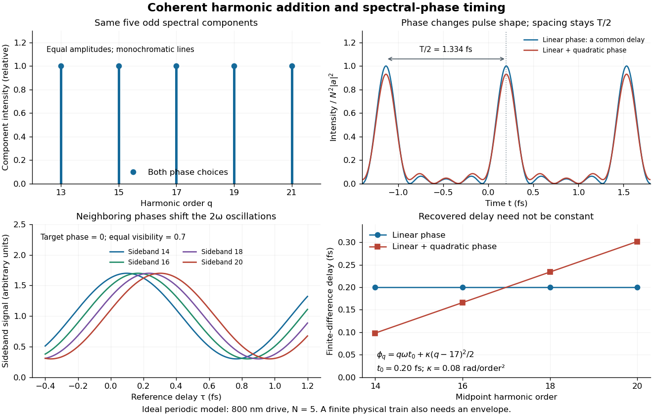
The infinite monochromatic sum is periodic forever and has infinite total energy. A real attosecond pulse train has a finite envelope and finite component linewidths. This calculation isolates coherent addition; it cannot describe an isolated burst or establish its contrast against satellites. As a further check, averaging $I(t)$ over one half-period gives $N|a{|}^2$ for any constant component spectral phases, because the cross terms integrate to zero by Fourier orthogonality. Spectral phase redistributes the light intensity in time while leaving that average fixed.

An isolated attosecond pulse has one dominant short burst within the observation window, with any satellite emission quantified. A broad optical spectrum alone cannot distinguish one burst from several. Selecting a generation interval and an appropriate spectral band can suppress neighboring bursts, but the resulting temporal contrast must still be tested.

For a simple calculation independent of any apparatus, let $\mathcal{E}(t)=f(t)+r{e}^{i\theta }f(t-\Delta )$, with two nonoverlapping copies of a short optical pulse. Its optical spectrum has intensityA satellite produces spectral fringes of angular spacing $2\pi /\Delta$ when the two bursts are coherent and resolved. For chosen field-amplitude ratio $r=0.2$, the satellite/main energy ratio is $r^2=0.04$, while fringe visibility is $2r/(1+r^2)\simeq 0.3846$. Weak satellite energy can thus leave substantial fringes. Averaging an uncontrolled $\theta$ removes the interference term without removing the satellite: absence of fringes alone does not prove isolation.

RABBITT measures adjacent harmonic spectral phases through two-photon photoionization. A weak delayed infrared reference opens two interfering paths to a shared photoelectron energy; the two-path attosecond phase reconstruction spells out the inference.

An original two-amplitude model makes the timing inference explicit. Use the spectral phase convention of the coherent harmonic pulse-train model, and define positive delay $\tau$ to retard the reference electric field. Let the amplitudes leading to the same final photoelectron state bewith real $b_{\pm }\ge 0$. Squaring their sum givesThe $2\omega$ oscillation comes from opposite signs of the reference photon's phase. For $\Delta {\varphi }_q=2\omega t_0$ and ${\delta }_q=0$, the signal peaks at $\tau =t_0$ modulo $T/2$. A fitted phase contains the target contribution ${\delta }_q$; setting it to zero is an assumption, not an observation. In an experiment, unobserved final channels can add as probabilities, so the displayed formula is one effective-channel idealization.

For a chosen example, impose $\Delta {\varphi }_q=0.80$ radians and ${\delta }_q=0.15$ radians at $800\mathrm{nm}$. The observed oscillation has argument $2\omega \tau -0.65$. Its peak shift is $0.1380\mathrm{fs}$, while the corrected finite-difference group delay is $\Delta {\varphi }_q/(2\omega )=0.1699\mathrm{fs}$. Ignoring the target contribution would bias the inferred delay by $-31.9$ attoseconds. These stipulated phases demonstrate a reconstruction error; they are not atomic calculations or measured delays.

Recovering all neighboring phase differences determines the component spectral phases up to an overall phase and the chosen timing origin, provided the oscillation phases are consistently unwrapped. Known component amplitudes then give a temporal field by a finite inverse Fourier transform. This is why measuring the optical spectrum alone is insufficient: it omits the very information that decides when constructive wave interference occurs.

Pierre Agostini's experiment illuminated an argon jet with an annular $800\mathrm{nm}$ beam. A pinhole removed the annulus; a tungsten-coated mirror relayed harmonics and weak central reference into another argon jet. A magnetic-bottle electron spectrometer used time of flight and microchannel plate detectors. Glass plates varied delay. Reference-on sidebands contrasted with reference-off peaks. Atomic-phase-corrected reconstruction yielded $250$-attosecond bursts.^[ref]

The two-path attosecond phase reconstruction explains the control's purpose: adding the reference opens an interference channel. Its fitted oscillation tests phase relationships under the weak-field and atomic-response model. It does not independently reveal every target phase or an arbitrary nonperiodic optical pulse.

Attosecond streaking uses a synchronized reference electric field to change a photoelectron's outgoing momentum. Scanning relative delay produces an energy-versus-delay distribution. A short emission interval samples only a small part of the reference cycle; a longer interval samples a range of kicks and can broaden or reshape the distribution.

For an explicit classical limit, use the electric dipole approximation and choose the magnetic vector potential $A(t)$ along the detection axis with $E(t)=-dA/dt$ and $A(\infty )=0$. Neglect the residual ion's Coulomb force. An Electron released at $t_i$ with mechanical momentum $p_0$ obeysIndeed, integrating $\dot{p}=-eE=e\dot{A}$ from release to the end of the field gives the stated minus sign. The useful clock variable here is $A$, rather than the instantaneous $E$ itself. If $A$ is nearly linear across a narrow emission window with temporal standard deviation ${\sigma }_t$, and initial momentum is sharp, thenThis local mapping fails near a zero of $E$, where first-order timing sensitivity vanishes. A real inversion must include the incident bandwidth, initial photoelectron distribution, collection angles and target–field response.

For an original dimensionless example in atomic units, choose $p_0=2$, $m=e=1$ and $A(t_i)=0.10$. Then $p_f=1.9$ and $K_f=1.805$, compared with initial kinetic energy $2$. Reversing $A$ gives $K_f=2.205$: the shifts are asymmetric because of the $A^2/2$ term. A measurement that keeps only the term linear in $A$ would miss $0.005$ in both cases.

The experiment involving Ferenc Krausz combined a subfemtosecond soft-X-ray pulse with a few-cycle visible electric field. Its delay-dependent krypton photoelectron spectra tested the field-controlled response. The reported pulse duration was $650\pm 150$ attoseconds. Changing delay compared the emitted Electron distributions at different reference phases; the spectral-width trace supplied a further duration-sensitive observable.^[ref]

The distinction from RABBITT is the measurement regime and reconstruction, rather than merely calling one trace a clock. The attosecond streaking momentum map is a limiting model; a finite-duration wave packet requires a quantum transition calculation. Inferring an emission delay also requires separating the illuminating pulse's spectral phase from the target response. The measurement supports time-dependent photoionization in a specified model, with no unique classical Electron trajectory inside an atomic orbital implied.