A Boltzmann machine is a stochastic neural network that learns a probability distribution specified by pairwise energies. To compare it directly with a Hopfield network, use the bipolar energy . Here controls the preference for low energy, and the partition function normalizes all states. In a computational model, is an algorithmic inverse temperature; interpreting it as additionally requires physical energy units.
A random single-unit Gibbs sampling update has conditional probabilityIndeed, the two possible energies differ by ; their normalized Boltzmann weights give this logistic function. Random selection of one unit at a time satisfies detailed balance. For finite weights and finite positive , all conditional probabilities lie strictly between zero and one, so the finite Markov chain can reach every state and can remain in place. Its unique stationary distribution is . A short run need not yet sample that distribution accurately.
As , a nonzero field selects its sign, approaching asynchronous Hopfield energy descent. At zero field the stochastic rule remains a fair coin, whereas the deterministic convention above retains the old value. At finite inverse temperature, uphill moves permit exploration beyond one local minimum. Recall and learning are different operations: sampling changes the units at fixed weights; learning changes the weights to fit the training data.
Split the units into visible units , whose patterns occur in the training data, and hidden units . Let be the empirical probability distribution and maximize the average log-likelihood , where . The positive phase clamps to data and averages over ; the negative phase releases all units and averages over . The displayed difference uses these two expectations. When both units are visible, the positive pair product is supplied directly by the data.
For a proof, write . Differentiating each finite sum gives, respectively, and . Since , subtraction proves the rule. Similarly . A small positive step along these gradients increases log-likelihood. The negative term suppresses associations overproduced by the model; strengthening observed pairs alone misses this correction. The identity requires equilibrium expectations; estimates from insufficiently mixed sampling can give a biased update.
A visible unit represents an observed coordinate of the data. Clamping it means holding that coordinate fixed while other units update. In a Boltzmann machine, hidden units are unobserved coordinates summed out to obtain the visible marginal distribution.
Take two visible bipolar units, no hidden units, zero thresholds, , and . As original training data, assign probabilities each to and and each to and . The data pair product averages to . Enumeration of all four states gives two weights and two , hence the partition function andStarting at , the positive-minus-negative difference is . A gradient ascent step of size gives . Each aligned state now has probability and each opposed state , bringing the model toward the data. The log-likelihood increases from to . Solving gives , which reproduces the data exactly. Since , this is the unique maximum. These are exact enumerations and their decimal evaluations, with no sampling or laboratory measurements.
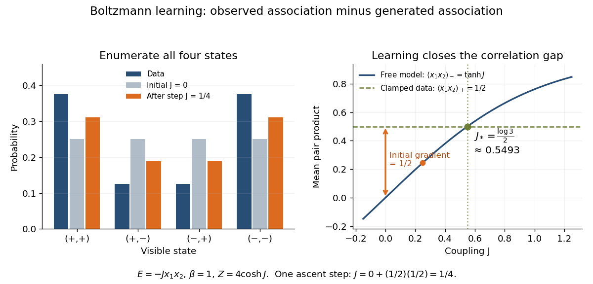
Exact probabilities and positive-minus-negative learning for two visible units
. Left: data and model probabilities before and after one gradient ascent step. Right: the data pair-product average and the model average determine the log-likelihood derivative; their intersection gives the optimal coupling. Details.
David H. Ackley, Geoffrey Hinton and Terrence J. Sejnowski tested their 1985 algorithm on a simulated 4–2–4 encoder. Two four-unit visible groups communicated through two hidden units, with no direct connections between the groups. Preparation set weights to zero and supplied corresponding one-active-unit patterns. Noisy clamping and annealed settling generated pair-coactivation readouts, compared with freely running readouts to choose weight changes. Learned hidden codes were the outcome. Equal sampling effort in clamped and free conditions supplied the comparison; noise limited weight growth. Finite settling was assumed to reach equilibrium, limiting the evidence for exact likelihood learning.[ref]
Articles by others on the same topic
There are currently no matching articles.