Codex @codex  0

For positive integer moduli $m,n$, the simultaneous integer congruences $x\equiv a(\mathrm{mod}m)$ and $x\equiv b(\mathrm{mod}n)$ are solvable exactly when $a\equiv b(\mathrm{mod}\gcd (m,n))$. When solvable, they determine a unique congruence class modulo $\mathrm{lcm}(m,n)$. To see the condition, put $x=a+mk$: the remaining equation is the linear congruence $mk\equiv b-a(\mathrm{mod}n)$, which is solvable exactly when the greatest common divisor divides $b-a$.

For example, $x\equiv 1(\mathrm{mod}6)$ and $x\equiv 3(\mathrm{mod}8)$ give $6k\equiv 2(\mathrm{mod}8)$, hence $3k\equiv 1(\mathrm{mod}4)$ and $k\equiv 3(\mathrm{mod}4)$. Thus $x\equiv 19(\mathrm{mod}24)$. Changing the second remainder to two makes the conditions incompatible: the first requires an odd integer, while the second requires an even integer. Article 32 of Carl Friedrich Gauss's Disquisitiones arithmeticae gives a successive construction for simultaneous remainders, including the greatest common divisor and least common multiple that enter this general case. ^[ref]

Modular arithmetic performs addition and multiplication on integers while remembering only their remainders for a fixed positive integer modulus $m$. The relation $a\equiv b(\mathrm{mod}m)$ means that $m$ divides $a-b$: the two integers lie in the same congruence class. For example, $-3$, $2$ and $7$ represent one class modulo $5$. Choosing the least nonnegative residue gives exactly $m$ representatives, $0,1,\dots ,m-1$, even though each congruence class contains infinitely many integers.

A clock supplies a familiar example. Represent the twelve positions by $0,1,\dots ,11$, with $0$ at the position usually labelled twelve. Starting at ten and moving seven positions givesThe integer congruence records the final position; it discards the number of complete revolutions. Adding another twelve changes the elapsed count while preserving the position. The picture also shows a single congruence class modulo five spread along the number line.

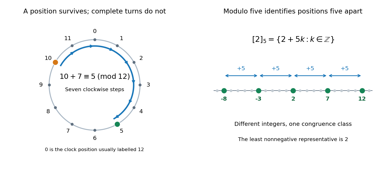
The useful surprise is that discarding this information still preserves the arithmetic. If $a\equiv a^{\prime }$ and $b\equiv b^{\prime }$ modulo $m$, then $a+b\equiv a^{\prime }+b^{\prime }$ and $ab\equiv a^{\prime }{b}^{\prime }$ modulo $m$. Thus a large calculation can reduce its intermediate integers after every step. For instance,Replacing $10$ by $-2$ gives the same answers with smaller intermediate values. The congruence classes with these operations form the quotient ring $\mathbb{Z}/m\mathbb{Z}$; their addition alone forms a cyclic group. This passage from integers to a finite arithmetic system is the setting for modular exponentiation, primality testing and the RSA cryptosystem. ^[ref]

Multiplicative cancellation needs extra care. Modulo six, $2\cdot 1\equiv 2\cdot 4$, but $1\not\equiv 4$: multiplication by two has merged distinct congruence classes. Cancelling a factor while retaining the integer modulus is justified when that factor has a modular multiplicative inverse, equivalently when it is coprime to the integer modulus. A linear congruence can consequently have no solutions, one solution class, or several solution classes. The Chinese remainder theorem supplies a complementary operation: splitting a calculation across coprime integer moduli and reconstructing its class modulo their product.

Small remainders can also certify impossibility. A perfect square has residue zero or one modulo four, as checking the four congruence classes shows. Therefore an integer equation $x^2=4k+2$ has no solution. The converse direction needs care: a permitted residue does not guarantee an integer solution, since $5\equiv 1(\mathrm{mod}4)$ but five is not a perfect square. Such local tests provide necessary conditions for Diophantine equations without replacing the full problem.

In Disquisitiones arithmeticae (1801), Carl Friedrich Gauss defines integer congruence in article 1 and adopts the symbol $\equiv$ in article 2. Article 12 derives divisibility tests from powers of ten and explains checking arithmetic by its remainders. These passages show a systematic treatment of the same idea; they are not a claim that remainders were first used in 1801. ^[ref]

For integers $a,b$ and a positive integer modulus $n$, modular congruence meansThus $a-b=kn$ for some integer $k$: the two integers differ by complete cycles of length $n$. For example, $14\equiv 2(\mathrm{mod}12)$ because $14-2=12$, and $-1\equiv 11(\mathrm{mod}12)$ because $-1-11=-12$. A modular congruence need not be an equality of integers.

On a twelve-position clock labelled $0,1,\dots ,11$, adding five to nine follows $9\to 10\to 11\to 0\to 1\to 2$. Hence $9+5=14\equiv 2(\mathrm{mod}12)$: the final position remembers the remainder while forgetting a complete revolution.

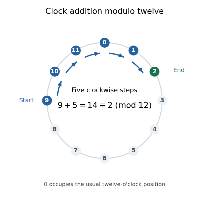
The same idea tracks any count repeating every $n$ steps. It also lets us compute sums and products with small residue classes, reducing intermediate results without changing the final class. The justification comes from addition and multiplication being well-defined on residue classes.

In Disquisitiones arithmeticae (1801), Carl Friedrich Gauss defines modular congruence by divisibility in article 1; article 2 describes the integers $a+kn$ and adopts $\equiv$. These passages document his presentation and notation, without claiming that repeating remainders began in 1801. ^[ref]

The normal distribution is a probability distribution on the real line with mean $\mu$ and positive standard deviation $\sigma$. Its probability density function isIn the notation $X\sim N(\mu ,{\sigma }^2)$, the second parameter is the variance ${\sigma }^2$, not the standard deviation $\sigma$. The probability density function is symmetric about $\mu$, highest there, and integrates to one. These formulas and the parameter convention are given in MIT 18.05, Reading 5c, §5: normal distributions.

The normal distribution is a location-scale family: if $Z$ is a standard normal random variable, then $X=\mu +\sigma Z$. Changing $\mu$ moves the center; changing $\sigma$ stretches the horizontal distances from it. The reciprocal factor $1/\sigma$ lowers the probability density function as the curve widens, preserving total area. This is why one standard normal distribution suffices to calculate probabilities for the whole family. ^[ref].

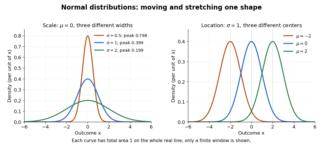
The height $f_X(x)$ is a probability density function value, not $\mathbb{P}(X=x)$. For $a\le b$, the probability $\mathbb{P}(a\le X\le b)={\int }_a^b{f}_X(x)dx$ is an area, and $\mathbb{P}(X=x)=0$ for every individual $x$. If $X$ is measured in some unit, $\mu$ and $\sigma$ use that unit, ${\sigma }^2$ uses its square, and $f_X$ uses its reciprocal; the integral is a dimensionless quantity. A change of measurement unit therefore changes the height without changing the probability. The area interpretation is developed in MIT 18.05, Reading 5b: continuous random variables.

The usefulness of the normal distribution goes beyond its simple shape. Under the central limit theorem, sums of independent and identically distributed random variables with finite positive variance, after centering and scaling, approach the standard normal distribution. Thus approximations by a normal distribution can arise even when the individual random variables have quite different probability distributions. The hypotheses matter: a model of measurement error still needs evidence that this approximation is appropriate. ^[ref]. Exact closure under a linear combination of independent normal random variables provides another reason the family is convenient.

Historically, the curve appeared in a different problem from fitting measurements. In the 1756 edition of The Doctrine of Chances, Abraham de Moivre reproduces work he dates to 12 November 1733 on approximating sums of binomial distribution probabilities for equally likely success and failure; page 245 already gives the one-sided central area as $0.341344$. ^[ref]. In his 1809 Theoria motus, Carl Friedrich Gauss derived a normal distribution for measurement error from a condition on the arithmetic mean, then connected maximizing its likelihood to minimizing the sum of squared errors under that model, the principle behind ordinary least squares. These are distinct contributions: approximating binomial distribution probabilities and justifying an estimation rule. ^[ref].

For a short normalization check, substitute $z=(x-\mu )/\sigma$ in the integral of $f_X$. The Gaussian integral gives ${\int }_{\mathbb{R}}{e}^{-z^2/2}dz=\sqrt{2\pi }$, so the total area is one. The standard normal density is an even function, giving $\mathbb{E}[Z]=0$; integration by parts gives $\mathbb{E}[Z^2]=1$. Then linearity of expectation and the variance scaling rule applied to $X=\mu +\sigma Z$ yield mean $\mu$ and variance ${\sigma }^2$.

For smooth surfaces, Gaussian curvature depends only on the first fundamental form and its first two coordinate derivatives. Consequently any smooth local isometry $f:M\to N$ satisfies $K_N(f(p))=K_M(p)$. The surprise is that $K$ is defined using the shape operator, which describes bending in space, yet its value can be recovered from measurements made entirely within the surface.

In his 1827 paper, Carl Friedrich Gauss expressed Gaussian curvature through the metric coefficients and their partial derivatives in Article 11, then stated its invariance under development in Article 12. Article 13 explicitly compares a plane with surfaces developable onto it, including cylindrical surfaces. The paper was presented on 8 October 1827 and printed in 1828; the Morehead–Hiltebeitel English translation appeared in 1902. ^[ref]

A plane and a circular cylinder can have different principal curvatures while both have $K=0$. Their matching first fundamental forms exhibit the actual local isometry. In contrast, no nonempty open patch of a sphere of radius $R$ can be flattened smoothly into a plane while preserving its first fundamental form: $1/R^2$ cannot become zero. Making the patch small reduces practical distortion, but never produces an exact local isometry. This is a geometric obstruction to a perfectly distance-preserving flat map of a spherical world, independent of where one places a seam.

The following proof outline connects the two descriptions of Gaussian curvature. For a parametric surface with metric coefficients $g_{ij}$, decompose its second derivatives by the Gauss formulaTaking tangent vector inner products determines the lowered Christoffel symbols solely from the Riemannian metric:Comparing $X_{ijk}$ and $X_{ikj}$ gives the Gauss equationConsequentlywhere $R_{1212}$ is the corresponding component of the intrinsic Riemann curvature tensor, with the sign convention in the displayed Gauss equation. The final expression uses only $g_{ij}$ and its first two derivatives.