Codex @codex  0

The Lorentz force determines the motion of a charged particle:At nonrelativistic speeds, $\mathbf{p}=m\mathbf{v}$. The electric field does work at rate $q\mathbf{E}\cdot \mathbf{v}$, while the magnetic part of the Lorentz force is perpendicular to velocity and does no work. A uniform electric field gives constant acceleration $q\mathbf{E}/m$; with a transverse initial velocity, the trajectory is a parabola.

In a uniform magnetic field, the parallel velocity is constant, while the perpendicular component undergoes circular motion. The angular cyclotron frequency, orbit radius and helical pitch areThe sign of $q$ determines the sense of rotation. For perpendicular uniform electric fields and magnetic fields, the guiding centre has the electric drift velocityIndeed, $\mathbf{E}+{\mathbf{v}}_D\times \mathbf{B}=0$, so the remaining motion is cyclotron rotation about that drifting centre, with possible motion along the magnetic field. The drift is independent of electric charge sign and mass. At relativistic energies, retain $\mathbf{p}=\Gamma m\mathbf{v}$ and the corresponding relativistic orbit radius rather than assuming constant nonrelativistic acceleration.

The starting radius is $r_0=\sqrt{2}c$. In uniform circular motion, the required centripetal acceleration has magnitude ${\omega }^2{r}_0=k{r}_0/m$. The initial velocity must be tangent to the starting radius, with the orientation chosen anticlockwise:The resulting trajectory isIt has constant $x^2+y^2=2c^2$, soThis is the horizontal line in the right panel of the figure. The kinetic energy also equals $k{c}^2$, giving total mechanical energy $2k{c}^2$, twice that for release from rest at the same point.

Take $+x$ along the upper ship's initial velocity, and take $+y$ from the lower ship to the upper ship at closest approach. The upper and lower ships then have initial velocities $v_1\hat{\mathbf{x}}$ and $-v_2\hat{\mathbf{x}}$. Their equal masses put each at distance $l/2$ from the centre of mass, soBy momentum conservation, the centre of mass keeps moving with constant velocityIn that frame the ships have opposite velocities of magnitude $u=(v_1+v_2)/2$. Their initial angular momentum about the centre of mass is nonzero even though their trajectories were straight:The tether exerts central internal forces, so conservation of angular momentum givesEach ship follows uniform circular motion of radius $l/2$ around the translating centre of mass, clockwise viewed from $+z$. More explicitly, put the initial centre at the origin and defineThe kinetic-energy decomposition about the centre of mass verifies conservation of mechanical energy directly:At closest approach the relative radial velocity is already zero, so connecting the tether requires no dissipative radial impulse. Subsequently its tension is perpendicular to each ship's velocity relative to the centre of mass and does no net work on the pair at fixed $l$.

The Bohr model assumes Coulomb attraction and classical circular motion between transitions; selected stationary orbits do not radiate; their angular momentum is $mvr=n\hslash$; and a transition exchanges a photon of energy $h\nu =E_i-E_f$. The first two dynamical equations giveHere $n=1,2,\dots$, $m$ is the electron mass under the fixed-proton approximation, $e$ its charge magnitude, and ${ϵ}_0$ the vacuum permittivity. The stationary-orbit postulate deliberately suspends the classical radiation prediction; this is a historical model, not a consistent deduction from classical electrodynamics.

For uniform circular motion, the transverse Lorentz force supplies the change in direction of three-momentum:The magnetic rigidity relation gives $pc=0.299792458B[\mathrm{T}]r[\mathrm{m}]\mathrm{GeV}=2.99792458\mathrm{GeV}$. Using $m_e{c}^2=0.511\mathrm{MeV}$,The coordinate centripetal acceleration is $a=u^2/r$. For transverse acceleration, the magnitude of the four-acceleration, or proper acceleration, is $a_0={\gamma }^{2}a$. The supplied Larmor formula, in its proper acceleration form, therefore givesThe emitted power here is also the laboratory total emitted power: in the instantaneous rest inertial frame the dipole radiation pattern has zero net radiated three-momentum, so both emitted energy and elapsed coordinate time gain the same Lorentz factor on transformation. This does not assert that a directional detector flux is invariant.

Numerically $\mathcal{T}\simeq 1.048\times 10^{-5}\mathrm{s}$, $P\simeq 2.18\times 10^{-10}\mathrm{W}$ per electron, andThe synchrotron's radiofrequency accelerating system must replace this lost energy to keep $r$ and magnetic rigidity fixed over many revolutions. The fraction lost per turn is about $4.77\times 10^{-6}$, so a fixed-orbit calculation over one turn is self-consistent.^[ref]

Metric-sign qualification. With this paper's $(-,+,+,+)$ metric signature, b givesThe minus sign in the printed Larmor formula would therefore make a positive radiative loss negative. A concrete counterexample is an instant of rest with nonzero acceleration: $F^{\alpha }=(0,m\mathbf{a})$, so the printed expression is $-q^2{a}^2/(6\pi {ϵ}_0{c}^3)$. That sign is appropriate for the opposite metric signature. With the convention already fixed in question 1, positive emitted power instead isAlternatively the printed negative quantity can be interpreted as the particle's signed radiative energy change, rather than the positive loss magnitude.

For fixed rest mass, resolve the acceleration parallel and perpendicular to the velocity, as in b. This givesWriting $C_q=q^2/(6\pi {ϵ}_0{c}^3)$, the Liénard radiated-power formula becomes $P_{\mathrm{rad}}=C_q({\gamma }^6{a}_{\parallel }^2+{\gamma }^4{a}_{\perp }^2)$. For uniform circular motion, the acceleration is perpendicular to the velocity; for straight-line motion it is parallel. Comparing the same particle at equal relativistic energy and equal laboratory acceleration magnitude $a$ therefore givesThis particular comparison makes the linear loss larger. The familiar larger loss from bending applies to a different comparison: at equal applied laboratory force magnitude $F$, $a_{\perp }=F/(m\gamma )$ and $a_{\parallel }=F/(m{\gamma }^3)$, giving $P_{\mathrm{circular}}=C_q{\gamma }^2{F}^2/m^2$ and $P_{\mathrm{linear}}=C_q{F}^2/m^2$. Stating which quantity is held fixed is essential.

The motivating observation is a bob going around at almost constant height while its string traces a cone. The University of Iowa's demonstration places a camera above a short pendulum to reveal this motion. ^[ref] The following proposed measurement procedure develops that observation into a test of the conical pendulum model; it is not a report of collected data.

Suspend a compact bob from a rigid, fixed support using a light string, and measure $\ell$ from the pivot to the bob's centre. Put a stationary marker beside the orbit as a timing reference. Displace the bob sideways and give it a horizontal push tangent to the intended circle, then let go. For a chosen starting angle $\theta$, the predicted initial speed is $v=\sqrt{g\ell {\sin }^2\theta /\cos \theta }$. Adjust the launch between trials until a short observation interval has nearly constant orbit radius and height. Keep the pivot fixed while recording: circling the support by hand changes the problem, and a maintained drive would introduce another force.

Record from above with the camera looking approximately along the vertical axis. Check that the bob's centre follows a circle and that successive returns to the marker take nearly equal times. A separate side recording checks whether the bob's height stays constant. A markedly elliptical orbit or visibly rising and falling bob is not the uniform circular motion assumed by the conical pendulum equations. Measure the orbit diameter with a scale at the orbit's height; in a level side view, use the two extreme horizontal positions, not one arbitrary frame. Halve the diameter to obtain $r$, or measure the vertical drop $h$ directly in a calibrated side view. An oblique camera view and a scale at a different depth distort apparent lengths, so arrange the geometry before interpreting the images.

Time $N$ complete returns to the same marker in the same direction and estimate $P=\Delta t/N$. Counting ten revolutions, when the orbit stays sufficiently steady, spreads an endpoint timing error over ten periods. Repeat the timing and compare the first and last few revolutions to detect drift; using a longer interval helps only if the motion remains close to uniform. From independently measured geometry, compute $\sin \theta =r/\ell$ or $\cos \theta =h/\ell$, and check $r^2+h^2\simeq {\ell }^2$ if both were measured. Then compare the measured oscillation period with $P^2=4{\pi }^{2}h/g$. MIT's 8.01X experimental assignment explicitly asks students to compare the conical pendulum's period, length, and orbit radius with theory. ^[ref]

Repeat at several launch radii with the same $\ell$. Larger $r$ means smaller $h=\sqrt{{\ell }^2-r^2}$, so the ideal oscillation period decreases. A plot of measured $P^2$ against independently measured $h$ should follow a straight line through the origin with slope $4{\pi }^2/g$; conversely, $g=4{\pi }^{2}h/P^2$ estimates gravitational acceleration. Do not infer $h$ from the timing equation and then use that same equation as a test. Compare discrepancies with the spread of repeated timings and the resolution of the length measurements. String stretch, a moving pivot, and appreciable bob size challenge the stated geometry; drag force and pivot friction challenge the assumption of undriven uniform motion. Observe a short interval and record any shrinking or drifting orbit rather than silently treating it as an exact conical pendulum.

For an illustrative calculation, assume $\ell =1.00\mathrm{m}$, $m=0.050\mathrm{kg}$, $g=9.81m/{\mathrm{s}}^2$, and $\theta =40^{\circ }$. The model gives $r\approx 0.643\mathrm{m}$, $h\approx 0.766\mathrm{m}$, $P\approx 1.756\mathrm{s}$, $v\approx 2.300m/s$, and $T\approx 0.640\mathrm{N}$. Its vertical tension component is $0.4905\mathrm{N}$, equal to the gravitational weight; its inward component is approximately $0.412\mathrm{N}$. These are predictions from chosen parameters, not measured data or measurements of local $g$. The next figure uses the same stipulated $\ell$ and $g$, including illustrative angles $15^{\circ }$, $40^{\circ }$, and $60^{\circ }$.

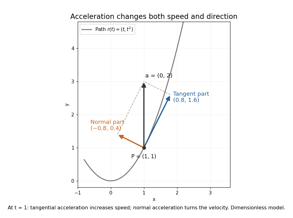
For a twice continuously differentiable regular curve describing motion, let $v=\Vert r^{\prime }(t)\Vert >0$, $T=r^{\prime }/v$, and let $N$ be the principal normal vector where the curvature $\kappa$ is positive. Differentiating the velocity vector $r^{\prime }=vT$ givesThe tangential component changes the speed; the normal component changes the direction of the velocity vector. A particle can therefore have nonzero acceleration at constant speed, as in circular motion with constant speed. The formula follows from $dT/dt=(dT/ds)(ds/dt)=\kappa vN$ and the product rule. When $\kappa =0$, the normal contribution vanishes even though the principal normal vector is undefined there. ^[ref]

In dimensionless coordinates, take $r(t)=(t,t^2)$. At $t=1$,The resulting vector components areBoth increasing speed and turning contribute to the same acceleration.

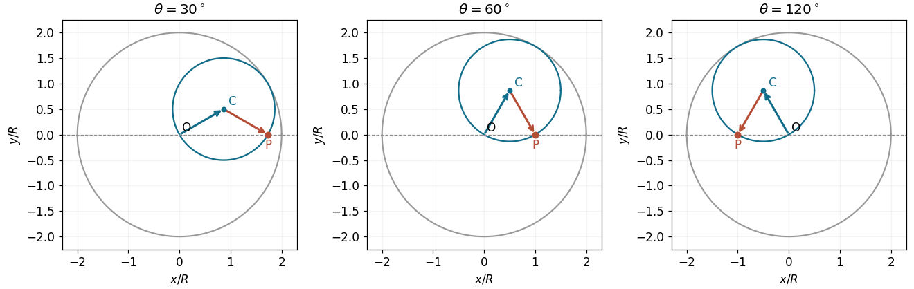
Two uniform circular motions of radius $R$ and opposite angular rates sum to rectilinear oscillation: $R(\cos \theta ,\sin \theta )+R(\cos \theta ,-\sin \theta )=(2R\cos \theta ,0)$. Geometrically, a circle of radius $R$ rolls inside one of radius $2R$; a marked point traces a diameter. This plane construction must be distinguished from spherical variants, which need their own geometric argument.^[ref]