Codex @codex  0

For a first-order system, it is important to specify the frame in which its coefficients are written. In the simple-pole convention intended here, a Fuchsian linear differential system has, at a finite singular point $a$,The residue is the matrix $R_a={\lim }_{z\to a}(z-a)A(z)$, computed entry by entry. Such a point is a regular singular point: on a sector, the coefficient bound $\Vert A(z)\Vert \le C/|z-a|$ and integration along rays give at most power growth of solutions. Intrinsically, a regular singular point means moderate power growth of all solutions on sectors, allowing logarithmic factors. This intrinsic definition is more general than requiring a simple coefficient pole in an arbitrary meromorphic frame.

For $A(z)=R/z$, a fundamental matrix on a chosen complex logarithm branch isDifferentiating the matrix exponential verifies ${\Phi }^{\prime }=R\Phi /z$. A counterclockwise circuit replaces $\log z$ by $\log z+2\pi i$, soThis is the residue and monodromy of a constant Fuchsian system. A change of solution basis conjugates $M$. Its eigenvalues are $e^{2\pi i\lambda }$ for the residue eigenvalues $\lambda$; a nontrivial Jordan block supplies the corresponding logarithmic terms in $z^R$. The monodromy does not uniquely recover $R$, since integer shifts of residue eigenvalues can leave their exponentials unchanged.

The coordinate-independent coefficient is the matrix-valued one-form $A(z)dz$. With $t=1/z$, its coefficient isBeing Fuchsian at infinity means $A(z)=O(z^{-1})$, while being ordinary there means $A(z)=O(z^{-2})$. If the finite simple poles are $a_1,\dots ,a_s$, subtract their principal parts:Each entry of $H$ is entire and tends to zero at infinity. Liouville's theorem therefore gives $H=0$. Expanding this partial fraction decomposition at infinity yieldsThus the sum of all residues, including the residue at infinity of the one-form, is zero. If infinity is ordinary, $R_{\infty }=0$ and the finite residues alone sum to zero. Treating $A$ merely as a scalar function of $z$, without transforming $dz$, would give the wrong infinity convention.

Put $\omega =e^{2\pi i/3}$. The possible finite singular points of $(B+zC)/(1-z^3)$ are $1,\omega ,{\omega }^2$, andA point $\zeta$ is removable exactly when $B+\zeta C=0$ as a matrix. At infinity,which is holomorphic at $t=0$. Consequently the actual set is $S=\{\zeta :{\zeta }^3=1,B+\zeta C\ne 0\}$, with $\{1,\omega ,{\omega }^2\}$ the generic set. The finite residues sum to zero, as follows also from ${\sum }_{{\zeta }^3=1}{\zeta }^{-1}={\sum }_{{\zeta }^3=1}{\zeta }^{-2}=0$.

Conversely, suppose a Fuchsian linear differential system has its finite singular points among these three roots and has no singularity at infinity. Then $Q(z)=(1-z^3)A(z)$ extends to an entire matrix function, and ordinariness at infinity gives $Q(z)=O(z)$. By the Cauchy estimate, each entry has zero derivatives of order two or higher, so $Q(z)=B+zC$. The same argument applies to any subset $S$, with additional cancellations at the omitted roots. This proves the requested normal form.

There is a genuine convention limitation: the normal form is not true under intrinsic regular singularity alone in an unrestricted frame. For example, if $N\ne 0$ and $N^2=0$, then $A(z)=N/(z-1{)}^2$ has fundamental matrix $I-N/(z-1)$. Its solutions have only power growth, so $1$ is intrinsically a regular singular point, and infinity is ordinary. Nevertheless its coefficient has a double pole and cannot equal $(B+zC)/(1-z^3)$. The simple-pole convention makes the preceding residue and normal-form assertions correct.

A branch of the complex logarithm must be specified to obtain a unique locus. First use the principal complex logarithm. Away from the negative real axis, write $z=r{e}^{i\theta }$ with $r>0$ and $-\pi <\theta <\pi$. Then the complex logarithms of $z$ and its complex conjugate are $\log r+i\theta$ and $\log r-i\theta$. Equating real and imaginary parts gives $\log r=\theta$. Consequently the principal-branch locus is the open segment of a logarithmic spiralThe origin is excluded because its complex logarithm does not exist. If the principal value is assigned argument $\pi$ on the negative real axis, a point there equals its own complex conjugate, so its principal complex logarithm would have to equal $i$ times itself. That forces the complex logarithm to be zero and cannot hold there; the endpoints remain excluded.

If the printed equation instead means that some values of the multivalued complex logarithms satisfy it, write those values as $\log r+it$ and $\log r+iu$, with $e^{it}=z/r$ and $e^{iu}=\overline{z}/r$. Equality gives $\log r=-u=t$, hence $u=-t$, which is compatible with conjugation. Every real $t$ is allowed. Under this interpretation the locus is the entire logarithmic spiral $z=e^{(1+i)t}$, $t\in \mathbb{R}$. The PDF does not choose between these branch conventions.

On the real line, Prohorov's theorem states that a sequence of probability measures is uniformly tight if and only if every subsequence has a further subsequence converging weakly to a probability measure. Here uniformly tight means that, for every $\epsilon >0$, some compact interval contains mass at least $1-\epsilon$ for every measure in the sequence. This is relative sequential compactness for weak convergence of probability measures, not merely the existence of one convergent subsequence.

We first prove the characteristic-function tail bound. Put $c_0=1-\sin 1>0$. For $y\ne 0$,At $y=0$ the expression is zero by continuity. If $|y|\ge \lambda$, the supplied elementary bound, with $t=|y|/\lambda$, makes it at least $c_0$. The integrand is nonnegative, so Tonelli's theorem yieldsThus one valid universal constant isThe estimate controls spatial tails using only the characteristic function near zero.

Apply it to each ${\mu }_n$. For fixed $\lambda$, pointwise convergence of the characteristic functions and the bound $|{\varphi }_n|\le 1$ allow dominated convergence on the finite integration interval, givingContinuity of a characteristic function and $\varphi (0)=1$ make the last expression tend to zero as $\lambda \to \infty$. Given $\epsilon >0$, choose $\lambda$ making it less than $\epsilon /2$; then for all sufficiently large $n$, the preceding tail is less than $\epsilon$. Enlarge the compact interval to handle the finitely many remaining probability measures. This proves uniform tightness of the whole sequence.

By Prohorov's theorem, every subsequence has a further weakly convergent subsequence, say with limit $\nu$. The real and imaginary parts of $e^{iuy}$ are bounded continuous functions, so along that subsequenceThe uniqueness theorem for characteristic functions implies $\nu =\mu$. All subsequential weak limits are therefore $\mu$. If the original sequence failed to converge weakly to $\mu$, a bounded continuous test function and a subsequence would keep its integrals a fixed distance from the limiting integral; a further weakly convergent subsequence would contradict that. HenceThis supplies the required proof of the Lévy continuity theorem in the stated case.

For the final request, the printed $Q$ is not defined; the intended function is $\varphi$, the characteristic function of a summand. We prove that ${\varphi }^{\prime }(0)=ia$ without assuming integrability. Write $Y_n=S_n/n$. Independence gives $\mathbb{E}{e}^{iu{Y}_n}=\varphi (u/n{)}^n$. Moreover convergence in probability to $a$ implies uniform convergence of these characteristic functions on each bounded frequency interval: for $|u|\le T$ and $\delta >0$,First let $n\to \infty$, then $\delta \downarrow 0$.

The potential logarithm-branch ambiguity needs to be resolved, not discarded. By continuity of $\varphi$ near zero, its principal complex logarithm is defined at $u/n$ for all $|u|\le 1$ and all large $n$, with value zero at $u=0$. Alsouniformly on $[-1,1]$, so $\mathrm{Log}{\Psi }_n(u)\to 0$ uniformly there. The two continuous logarithms differ by an integer multiple of $2\pi i$:That integer is continuous in $u$ and zero at zero, hence identically zero. ConsequentlyFor arbitrary nonzero $h\to 0$, take $n=\lfloor 1/|h|\rfloor$ and $u=nh$. Eventually $1/2\le |u|\le 1$, so dividing the preceding error by $u$ shows $\mathrm{Log}\varphi (h)/h\to ia$. Exponentiating at zero proves the derivative forced by the weak law:This is the weak law forces a characteristic-function derivative argument. Its estimates use bounded exponentials, not $\mathbb{E}|X_1|$. If $X_1$ is integrable, dominated convergence permits differentiation inside the expectation and gives ${\varphi }^{\prime }(0)=i\mathbb{E}{X}_1$, so then $a=\mathbb{E}{X}_1$.

Absolute integrability is genuinely unnecessary. For an explicit weak law without an absolute first moment, take a symmetric variable withwith mass $1-1/e$ at zero and no mass with $0<|X|<e$. This is a valid law: the specified tail decreases from $1/e$ to zero, and its derivative defines the continuous part beyond $e$. Its absolute first moment is infinite because ${\int }_e^{\infty }dx/(x\log x)=\infty$. For independent copies, set $Y_{n,j}=X_j{1}_{\{|X_j|\le n\}}$. Symmetry gives $\mathbb{E}{Y}_{n,j}=0$, and integration of the tail givesFor the last estimate, split the integral at $\sqrt{n}$; the initial part is $O(\sqrt{n})$ and the remainder is at most $2n/\log n$, apart from a fixed initial constant. Chebyshev's inequality now gives $n^{-1}{\sum }_{j\le n}{Y}_{n,j}\to 0$ in probability. The probability that any truncation changes a summand is at most $n\mathbb{P}(|X|>n)=1/\log n\to 0$, so $S_n/n\to 0$ in probability although $\mathbb{E}|X|=\infty$. The derivative is zero, but the usual expectation of $X$ does not exist.

If either the positive or negative part is integrable, the finite weak-law limit does force full integrability. For example, if $\mathbb{E}{X}^{-}<\infty$, then $X\wedge A$ is integrable and its sample averages have the weak law of large numbers limit $\mathbb{E}(X\wedge A)$. Since they are bounded above by the original averages, $\mathbb{E}(X\wedge A)\le a$ for every $A$. Letting $A\to \infty$ shows $\mathbb{E}{X}^{+}<\infty$. The symmetric argument handles the other one-sided hypothesis. The nonintegrable example necessarily has both one-sided expectations infinite.

For a nonzero complex number, write $z=r{e}^{i\theta }$ with $r=|z|>0$ and principal complex argument $-\pi <\theta \le \pi$. The principal complex logarithm and corresponding complex exponentiation areThe value at zero is not defined by this formula. The choice of complex argument matters: these are single-valued principal powers, rather than all values of a multivalued complex logarithm.

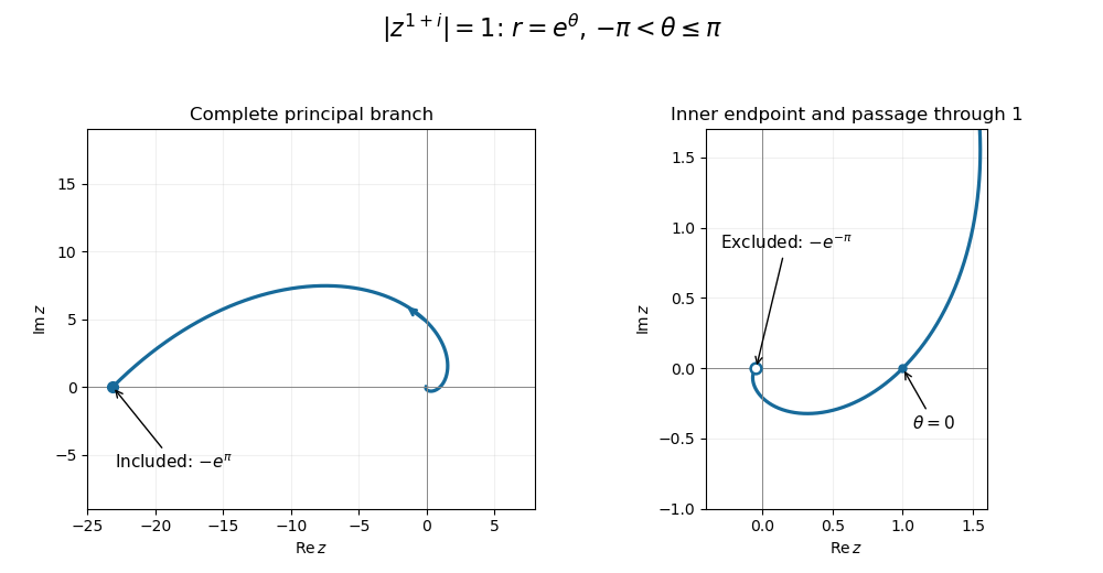
For the requested sketch, $(1+i)\mathrm{Log}z=(\log r-\theta )+i(\log r+\theta )$. Its complex exponential has complex modulus $e^{\log r-\theta }$, soThis is one turn of a logarithmic spiral, with increasing radius as the polar angle increases. It passes through $1$ at $\theta =0$, approaches the excluded endpoint $-e^{-\pi }$ from below the negative real axis, and ends at the included endpoint $-e^{\pi }$ from above that axis. The endpoint distinction follows from the chosen principal complex argument.

With $t=1-x^2$ the chain rule gives $y^{\prime }=-2x{u}^{\prime }$ and $y^{\prime \prime }=-2u^{\prime }+4x^2{u}^{\prime \prime }$. Substitution, initially for $x>0$, givesThe transformed coefficients are $P(t)=1/t$ and $Q(t)=1/[4t(1-t)]$. At $t=0$, both $tP$ and $t^{2}Q$ are analytic; at $t=1$, both $(t-1)P$ and $(t-1{)}^{2}Q$ are analytic. Each point is singular because a normalized coefficient has a pole, but satisfies the regular singular point criterion for a second-order equation. Thus both points are regular singular points.

For a Frobenius method substitution $u=t^{\rho }{\sum }_{n\ge 0}{a}_n{t}^n$, the lowest power gives the indicial equationThe repeated indicial root is zero. Setting $\rho =0$ and equating the coefficient of $t^n$ givesConsequently the analytic power-series solution of a differential equation isTaking $a_0=2\pi$ reproduces the ellipse perimeter expansion.

For a second independent solution, normalize $u_1(0)=1$. Reduction of order and $P=1/t$ giveSince $u_1(s{)}^{-2}=1+O(s)$, this has the Logarithmic Frobenius solution formThe logarithm is $\log |t|$ on the real negative side, or a chosen complex logarithm on a slit complex neighborhood. Its nonzero logarithmic coefficient establishes independence. The physical perimeter is finite at $t=0$, so it selects the analytic branch rather than this logarithmic one.

Let $w$ denote the value of the complex logarithm used in the equation. Factoring $w^2+{\pi }^2/4$ gives $w=i\pi /2$ or $w=-i\pi /2$. Since $z=e^w$, the complete answer isThe principal complex logarithm takes exactly these values at $i$ and $-i$, so both are solutions with that convention. If the complex logarithm is interpreted as multivalued, the same answer holds in the sense that a logarithm value satisfies the equation. The equation is not an assertion that every logarithm value of these numbers has the stated square.

Use the scattering potential convention $V=k_0^2(n^2-1)$. With time dependence $e^{-i\omega t}$ the outgoing Green function is $G_0(r,r^{\prime })=e^{i{k}_0|r-r^{\prime }|}/(4\pi |r-r^{\prime }|)$ and satisfies $(\Delta +k_0^2)G_0=-\delta$. The total-field Lippmann-Schwinger equation isReplacing the field in the integral by the incident field gives the first Born approximation for scalar wave scattering:For the first Rytov approximation, write $\psi ={\psi }_0{e}^{\chi }$ on a region where the incident field is nonzero and a continuous complex logarithm can be chosen. The logarithmic wave perturbation equation isThe last dot product is bilinear, not a squared modulus. Dropping it leaves a linear equation for ${\chi }_1$. Multiplication by ${\psi }_0$ shows that ${\psi }_0{\chi }_1$ satisfies the same outgoing inhomogeneous Helmholtz equation as ${\psi }_1$. HenceIntroduce a small multiplier $\lambda$ on $V$. Then ${\psi }_1=O(\lambda )$ andThe two total-field approximations agree to first order. Exponentiating the first logarithmic wave perturbation does not supply the generally missing second-order Born series contribution.

We give a quantitative construction for the whole open set, including the case of infinitely many component intervals. Pointwise divergence at a single point is insufficient here. Write $z=e^{2\pi it}$ and use normalized measure on $\mathbb{T}$.

First let $K$ be a finite union of closed arcs with $|K|\le 3\epsilon$, where $\epsilon$ is small. Choose a smooth function nonnegative function $u$, equal to one on $K$, with $u\le 1$ and $\eta :=\int u\le 6\epsilon$. This follows by making the transition regions around the finitely many arc endpoints sufficiently short. Define the analytic Herglotz integralIts real part is $(\eta +P[u](z))/(2\eta )>0$, where $P[u]$ is the disk Poisson integral, and $G(0)=1$. Smoothness of $u$ makes $G$ continuous and smooth function up to the circle; on $K$ its boundary real part is at least $1/(2\eta )$. The branch $H=\log G$ therefore has $H(0)=0$ andThe complex logarithm has no branch problem because $G$ lies in the right half-plane. Its smooth function boundary values give absolutely summable Taylor coefficients. Choose an analytic polynomial $A$, with zero constant coefficient, uniformly within $1/4$ of $H$ on the closed disk. Put $P(t)=\mathrm{Im}A(e^{2\pi it})/\pi$. Then $\Vert P{\Vert }_{\infty }\le 1/2+1/(4\pi )<1$.

If $D=\mathrm{deg}A$ and $m>D$, the modulated trigonometric polynomial $Q(t)=e^{2\pi imt}P(t)$ has spectrum in $[m-D,m+D]$. A sharp Fourier partial sum at $m$ selects exactly the negative-frequency half of $P$, since $A(0)=0$:Consequently, for every $t\in K$,The carrier frequency $m$ can be arbitrarily large. This compact-set Fourier amplification lemma uses a bounded imaginary part to obtain a large one-sided Fourier multiplier; no assertion about pointwise divergence is used.

Now let $E$ be any open set of measure $\delta$. DefineIf this is zero take $f=0$. Otherwise choose a decreasing sequence ${\delta }_j\downarrow 0$, with ${\delta }_1=\delta$, so small for $j\ge 2$ thatFor $j=1$ this inequality also holds: $B(\delta )>4$ and $B(\delta )/2\ge B(\delta )/4+1$. Let $L_j$ be an increasing compact exhaustion of $E$.

Using compact batching of a small open set, we recursively choose finite closed-arc unions $K_j\subset E$, of measure at most $3{\delta }_j$, such that $L_j$ is covered by the interiors of $K_1,\dots ,K_j$ andHere is the measure-theoretic justification. At step $j$, the uncovered portion has measure at most ${\delta }_j$. Its intersection with $L_j$ after removing the previously covered interiors is compact, and can be covered by finitely many closed arcs lying in $E$ with total length at most ${\delta }_j$ plus an arbitrarily small excess. By inner regularity of Lebesgue measure, a further compact subset of the uncovered open portion captures all but ${\delta }_{j+1}$ of its measure; cover it similarly. The combined finite arc union has length at most $3{\delta }_j$. This both covers the outstanding part of $L_j$ and ensures the next remainder estimate. In particular $E\subset {\bigcup }_j{K}_j$.

Apply the finite-arc construction to $K_j$ to get $P_j$ of degree $D_j$. Choose carriers $m_j$ recursively so that the bands $[m_j-D_j,m_j+D_j]$ are positive and strictly ordered with no overlap. SetThe frequency-separated Fourier block series and the Weierstrass M-test give a continuous complex-valued function with $\Vert f{\Vert }_{\infty }\le {\sum }_j{2}^{-j}=1$. At the cutoff $m_j$, all earlier bands have been included in full and every later band is absent. Thus on $K_j$,Every point of $E$ lies in some $K_j$, soValues of $\psi$ outside $0<\delta \le 1$ may be defined arbitrarily. The construction handles an arbitrary open set, not just one point or a finite collection of intervals. It also prevents cancellation explicitly: earlier bands contribute a bounded complete sum, and later bands contribute nothing at the chosen cutoff.

For fixed $u$, write $h(t)={\phi }_{X_t}(u)$. Independent increments and stationary increments giveThe preceding part gives continuity. Also $h$ never vanishes: if $h(t_0)=0$ with $t_0>0$, then $h(t_0/m{)}^m=0$ for every positive integer $m$, contradicting $h(t_0/m)\to 1$.

Here is a direct proof of the exponential form of Lévy characteristic functions. Choose $a>0$ small enough that $|h(t)-1|<1/2$ on $[0,a]$. The principal complex logarithm gives a continuous $L(t)=\log h(t)$ there, with $L(0)=0$. For $s,t\ge 0$ with $s+t\le a$, the multiplicative identity impliesThis difference is continuous on the connected triangle of allowed $(s,t)$ and equals zero at $(0,0)$, so it is identically zero. Thus $L$ satisfies the additive Cauchy functional equation locally. Subdivision gives $L(a/m)=L(a)/m$ and $L(ka/m)=kL(a)/m$; continuity then gives $L(t)=tL(a)/a$ for every $t\in [0,a]$.

Define $\eta (u)=L(a)/a$. For any $t\ge 0$, choose an integer $m$ with $t/m\le a$; thenThe coefficient is unique: if two coefficients give the same exponential for every $t\ge 0$, their derivatives at zero agree. In particular $\eta (0)=0$, and $\mathrm{Re}\eta (u)\le 0$ follows from $|h(t)|\le 1$. The characteristic exponent of a Lévy process has therefore been obtained from first principles, without invoking the Lévy–Khintchine formula.

Use $U_t=2W_t$ and write $Z_t=X_t+i{Y}_t$ up to its interior-point swallowing time for a Loewner chain $T_z$. The Chordal Loewner equation givesThe branch of the complex logarithm with argument in $(0,\pi )$ is well-defined while $t<T_z$. The Itô formula yields the crucial cancellationThe $2/Z_t^2$ drift is cancelled by the quadratic variation term, because $\kappa =4$. Thus both $L_t=\log |Z_t|$ and ${\theta }_t=\arg Z_t$ are continuous local martingales, withThis is the logarithmic martingale for SLE4.

We justify absence of a finite swallowing time rather than presuming that the logarithm survives forever. On a finite horizon $H$, $0<Y_t\le \mathrm{Im}z$. Also $|X_t|$ is bounded pathwise before $T_z\wedge H$. Indeed, while $|X_t|\ge 1$ its drift $2X_t/|Z_t{|}^2$ has absolute value at most $2$; on each excursion outside $[-1,1]$, integrate from its starting point and bound the Brownian oscillation on $[0,H]$. For example,Therefore $L_t$ is bounded above pathwise on this interval.

Suppose $T_z\le H$. By the Dambis-Dubins-Schwarz theorem, $L$ is a Brownian motion run at its own quadratic variation. If that clock diverged as $t\uparrow T_z$, Brownian oscillation would make $L$ unbounded above, contradicting the preceding bound. The one-sided bound criterion for a martingale clock therefore gives a finite clock limit and a finite real limit for $L_t$. Hence $|Z_t|$ is bounded away from zero near $T_z$.

Now $Y_t=Y_0\exp (-2{\int }_0^t|Z_s{|}^{-2}ds)$ has a strictly positive limit at $T_z$. The drift in $X$ is integrable there, so continuity of $W$ gives a finite limit for $X$ as well. The limiting point is in $\mathbb{H}$ and away from the Loewner driver singularity, and the differential equation extends past $T_z$, a contradiction. Thus $T_z=\infty$ almost surely. A point of the Loewner trace at a finite time belongs to that time's hull, soThis proves the fixed-interior-point avoidance of SLE4 without using simplicity as an input.

The angle remains in $(0,\pi )$ at all finite times. The bounded local martingale criterion upgrades its local martingale equation to a genuine martingale:In particular this is the SLE4 angle martingale, and it converges almost surely and in $L^1$ by bounded martingale convergence theorem.

It remains to identify the limiting angle using the assumed simple path tending to infinity. Orient that path from $0$ to infinity. Its left component is the one adjacent to the negative real half-axis. Under $g_t$, the left boundary of the slit domain maps to $(-\infty ,U_t)$ and the right boundary to $(U_t,\infty )$. The harmonic measure of the former as seen from $z$ isThis follows by conformal invariance of planar Brownian motion: in the upper half-plane, $\arg (w-U_t)/\pi$ is the bounded harmonic function with values $1$ on the left half-axis and $0$ on the right.

To justify the limiting boundary classification, condition on a simple proper realization of the path and use an independent planar Brownian motion from $z$. It exits the upper half-plane in finite time almost surely, so its path up to that time is compact. The curve tends to infinity, so its intersection with this compact set is contained in a finite initial curve segment. Once that segment has been drawn, the Brownian path exits the slit domain through its left boundary exactly when $z$ is in the final left component: a path from that component cannot reach the right boundary without crossing the curve, and the reverse assertion holds on the right. Endpoints have zero harmonic measure. Bounded convergence of these exit indicators provesTaking expectations in the bounded angle martingale gives the SLE4 left-passage probabilityFor the imaginary axis it is $1/2$; near the negative real axis it tends to $1$, fixing the orientation of “left”.

Use the principal complex logarithm in the upper half-plane. Deform the interval upward into a half-strip: the vertical side at zero is traversed upward, and the side at one downward. The top side vanishes exponentially; a small indentation at zero contributes $O(r|\log r|)$ and vanishes. Thus the contour deformation gives the exact representation, for $x>0$,Since $\log (is)=\log s+i\pi /2$, scaling $u=xs$ and using the integral defining Euler's constant givesFor the second endpoint, $\log (1+is)=is+s^2/2+O(s^3)$. Watson's lemma, or integration of these powers against $e^{-xs}$ with an exponentially small tail, yieldsIn particular the required first terms areThe two different endpoint scales come from the logarithmic singularity at zero and the simple zero of the amplitude at one.

Analytic continuation extends a holomorphic function by holomorphic elements agreeing on overlaps; along a path, a chain of overlapping neighbourhoods transports the initial element. The identity theorem makes compatible continuation unique on connected overlaps, although different paths can lead to different branches.

Choose the principal complex logarithm and the slit domain $D=\mathbb{C}\setminus [1,\infty )$. On $D$, the functionis holomorphic, with the removable value $h(0)=1$. The domain $D$ is simply connected, so $h$ has a primitive and its integral from $0$ to $z$ is independent of the path in $D$. For $|z|<1$, the uniformly convergent power series on compact subdiscs givesTherefore $f$ is a single-valued analytic continuation of the dilogarithm to $\mathbb{C}\setminus [1,\infty )$. The apparent problem at $0$ is removable; $1$ is a genuine branch point, even though the function has a finite one-sided limit there, because its derivative has a logarithmic singularity. Other cuts from $1$ to infinity give corresponding branches.

ChooseIt is holomorphic on the right half-plane with derivative $1/z\ne 0$, and its inverse $z=e^w$ has positive real part precisely for $|\mathrm{Im}w|<\pi /2$. Thus this branch of the complex logarithm is a conformal bijection onto $S$.

Write $A_n=n^{-1}{\sum }_{j=1}^n{X}_j$ and $\phi (t)=\mathbb{E}{e}^{it{X}_1}$. The given two-sided limit $|f(u)|/u\to 0$ implies $|f(u)|/|u|\to 0$, so $f(u)=o(|u|)$. For each fixed real $t$, independence and the characteristic function of a sum of independent variables giveSet $z_n=iat/n+f(t/n)$. For $t\ne 0$, $n{z}_n\to iat$ and $z_n=O(n^{-1})$. The local Taylor expansion of the complex logarithm at $1$ givesThus $\mathbb{E}{e}^{it{A}_n}\to e^{iat}$; at $t=0$ the identity is immediate. The limit is continuous at zero and is the characteristic function of the constant random variable $a$. The Lévy continuity theorem proves the weak law from a characteristic-function expansion:No integrability hypothesis has been used. The conclusion is also convergence in probability by (d)'s convergence in distribution to a constant implies convergence in probability. If the word “constant” were to allow complex $a$, the characteristic function symmetry $\phi (-t)=\overline{\phi (t)}$ forces $a=\overline{a}$, so it is necessarily real.

Write $z=r{e}^{i\theta }$ with $r>0$ and $0\le \theta <2\pi$, and write $w=u+iv$. Sincewe haveThus the inverse of the exponential is the infinitely valued complex logarithmFor the angle convention in the question, its principal value is

All values of the complex logarithm areBecause $x>0$, one may take the complex argument $\arg z=\arctan (y/x)$. Consequently

Rouché's theorem states that if $g$ and $h$ are holomorphic functions on a neighbourhood of the closure of a bounded domain andon its positively oriented boundary, then $g$ and $g+h$ have the same number of zeros in the domain, counted with multiplicity.

The Open mapping theorem states that a nonconstant holomorphic function on a domain maps every open subset to an open subset. To prove it, fix $z_0$ and put $w_0=f(z_0)$. By the identity theorem, the zeros of $f-w_0$ are isolated. Choose $r>0$ so that the closed disc $\overline{D(z_0,r)}$ lies in the domain and $z_0$ is the only zero of $f-w_0$ in that disc. ThenWhenever $|w-w_0|<\delta$, the constant $w_0-w$ has modulus smaller than $f-w_0$ on the circle. The Rouche theorem therefore says thathas the same positive number of zeros in the disc as $f-w_0$. Thus every $w\in D(w_0,\delta )$ lies in the image of $f$, proving that the image is open.

If $|f|$ had a local maximum at $z_0$, take a small open disc $D$ on which $|f(z)|\le |f(z_0)|$. The restriction of $f$ to $D$ cannot be constant, since the identity theorem would then make $f$ constant on the whole domain. The complex open mapping theorem says that $f(D)$ is an open neighbourhood of $f(z_0)$, and such a neighbourhood contains points of modulus greater than $|f(z_0)|$, a contradiction. This proves the maximum modulus principle from the complex open mapping theorem.

Now let $\Omega$ be bounded. Its closure is compact, so the continuous function $|f|$ attains a maximum there. If $f$ is nonconstant, the maximum modulus principle excludes an interior maximum; if $f$ is constant, the claimed bound is immediate. Hencewhich is the maximum modulus principle on a bounded domain.

Finally let $\Omega =\{z:\mathrm{Re}z>1\}$ and suppose $|f|\le K$ throughout $\overline{\Omega }$. Fix $z_0\in \Omega$. The principal complex logarithm is holomorphic on the right half-plane, so for each positive integer $n$ the functionis holomorphic on $\Omega$ and continuous on its closure. Given $\epsilon >0$, choose $R>|z_0|$ so large thatApply the bounded-domain result to $g_n$ on $\Omega \cap D(0,R)$. On the vertical part of the boundary, $|z|\ge 1$ and hence $|g_n(z)|\le M$. On the circular part,It follows thatLetting $n\to \infty$ and then $\epsilon \to 0$ gives $|f(z_0)|\le M$. Since $z_0$ was arbitrary, this proves the bounded half-plane maximum principle.

The boundedness assumption is necessary. The functionis holomorphic on $\Omega$ and continuous on its closure, and $|f(1+iy)|=e$ on the boundary, but $|f(x)|=e^x$ is unbounded for real $x>1$. Thus the boundary estimate does not control an unbounded holomorphic function on this unbounded domain.

The number $i{e}^{i\varphi }$ has modulus one and argument $\varphi +\pi /2$ modulo $2\pi$. Therefore its complex logarithm has valuesEvery value has real part zero. For the principal complex logarithm, choose the unique integer giving imaginary part in $(-\pi ,\pi ]$. The unwrapped value $\varphi +\pi /2$ is the principal imaginary part only when it already lies in that interval.