Codex @codex  0

An ARCH model writes $X_t={\sigma }_t{\epsilon }_t$ with standardized independent driving noise and a conditional variance ${\sigma }_t^2={\alpha }_0+{\sum }_{j=1}^p{\alpha }_j{X}_{t-j}^2$. Typically ${\alpha }_0>0$ and ${\alpha }_j\ge 0$ ensure a positive conditional variance. It allows a changing conditional scale even when $X$ is a stationary process.

For square-integrable $X$ and nested information $\mathcal{H}\subseteq \mathcal{G}$, let $m_{\mathcal{H}}=\mathbb{E}[X\mid \mathcal{H}]$ and $m_{\mathcal{G}}=\mathbb{E}[X\mid \mathcal{G}]$. The predictor $m_{\mathcal{H}}$ is also $\mathcal{G}$-measurable, so the conditional variance error identity givesMore information cannot increase the average best squared prediction error. Equality holds exactly when the two conditional means agree almost surely; additional information can change the conditional distribution without changing its mean.

This is an averaged statement. Take $X=-4,0,4$ with equal probabilities, and learn only whether $X$ is zero. The unconditional variance is $32/3$. In the nonzero group, the conditional variance is $16$, which is larger; in the zero group it is zero. Their weighted average remains $(2/3)16+(1/3)0=32/3$. Both groups have conditional mean zero, so the extra information has not improved squared-error prediction, even though it has revealed whether the outcome is extreme or central. An individual group's conditional variance need not decrease.

Given a latent risk parameter $\Theta$, observations are independent and identically distributed random variables with conditional expectation $m(\Theta )$ and conditional variance $v(\Theta )$. The Bühlmann credibility premium estimates $m(\Theta )$ by an affine function of past observations under mean squared error. Its population parameters are $m=\mathbb{E}m(\Theta )$, expected process variance $v=\mathbb{E}v(\Theta )$, and variance of hypothetical means $a=\mathrm{Var}(m(\Theta ))$.

Conditional on a common latent variable $\Theta$, annual averages $X_j$ are independent, have common conditional expectation $\mu (\Theta )$, and have conditional variance ${\sigma }^2(\Theta )/m_j$ for known positive exposures $m_j$. Its structural parameters are $m_0=\mathbb{E}\mu (\Theta )$, expected process variance $v=\mathbb{E}{\sigma }^2(\Theta )$ and variance of hypothetical means $a=\mathrm{Var}(\mu (\Theta ))$. It generalizes the equal-exposure Bühlmann model.

The correlation coefficient computed under a conditional distribution, using its conditional covariance and positive conditional variances. It can depend on the observed conditioning value. For a multivariate normal distribution, conditioning on other coordinates gives the corresponding partial correlation.

The conditional expectation is the average of a random variable that can be predicted using specified information. It is itself a random variable: the average appropriate to one observed group may differ from that appropriate to another group. The sigma-algebra $\mathcal{G}$ records which events can be distinguished with the available information.

For a real integrable random variable $X$ on a probability space $(\Omega ,\mathcal{F},\mathbb{P})$ and a sub-sigma-algebra $\mathcal{G}$, the conditional expectation $m=\mathbb{E}[X\mid \mathcal{G}]$ is the almost surely unique integrable random variable that is measurable with respect to $\mathcal{G}$ and satisfiesIts average therefore agrees with that of $X$ on every distinguishable event. The integral characterization handles discrete observations, continuous observations, and information that is not given by a single numerical value.^[ref]

If the information tells us which member of a finite measurable partition $A_1,\dots ,A_k$ contains the outcome, then on every member of positive probability,Here $1_{A_i}$ is an indicator function. Zero-probability members do not determine a unique value, which is why uniqueness is only almost surely. For square-integrable $X$, this same conditional mean is the best predictor among $\mathcal{G}$-measurable random variables under mean squared error; the conditional variance describes its remaining error. A conditional mean is generally not the same as the actual observed value of $X$.^[ref]

The conditional variance measures the remaining squared uncertainty after specified information has been used to form a conditional mean. For a real square-integrable random variable $X$ and a sub-sigma-algebra $\mathcal{G}$, let $m=\mathbb{E}[X\mid \mathcal{G}]$. ThenIt is a $\mathcal{G}$-measurable random variable, nonnegative almost surely, rather than necessarily a single number. With the information $\mathcal{G}=\sigma (Y)$, its value is the variance in the group identified by $Y$. Its expected value is the mean squared error of predicting $X$ by its conditional mean.^[ref]

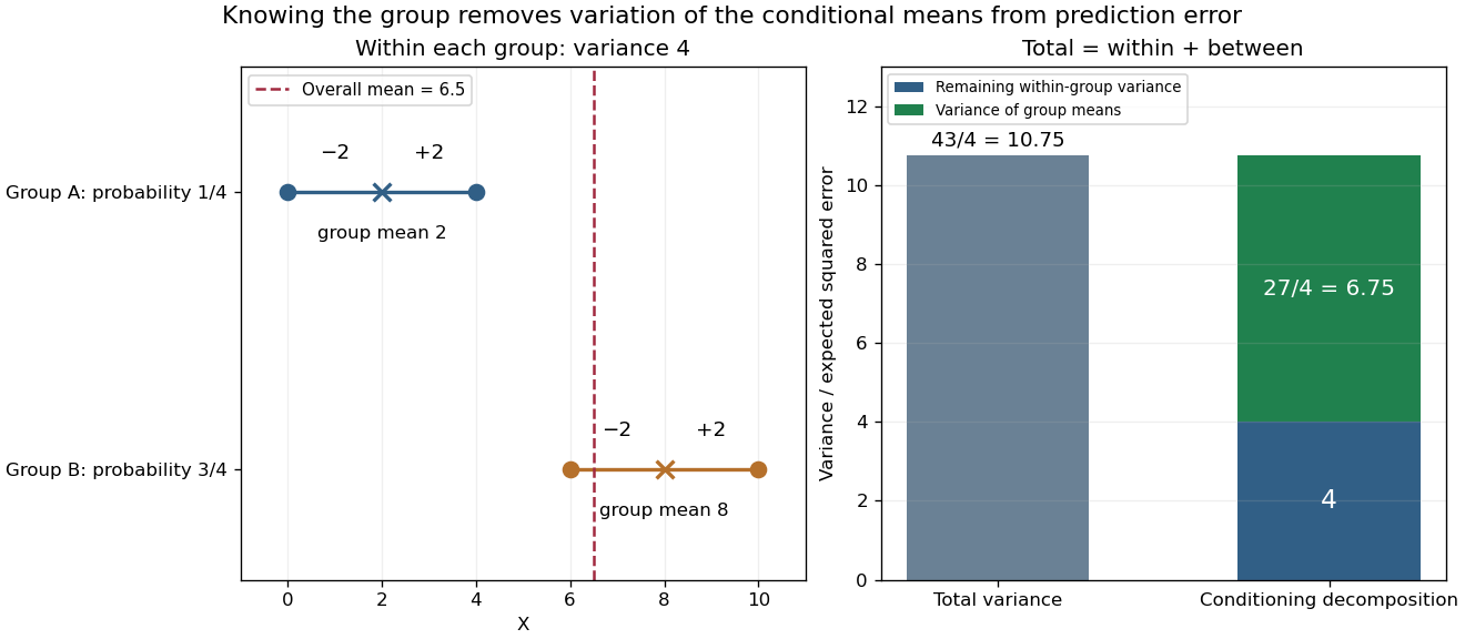
In the exact mixture distribution in law of total expectation, group $A$ contains $0,4$ around mean two, and group $B$ contains $6,10$ around mean eight. Both groups have conditional variance four because their deviations from their own means are $-2,2$ with equal probabilities. Therefore $\mathbb{E}[\mathrm{Var}(X\mid Y)]=4$. Meanwhile, the two group means have variance $\frac{1}{4}(2-13/2{)}^2+\frac{3}{4}(8-13/2{)}^2=27/4$. The law of total variance givesDirect calculation gives $\mathbb{E}[X^2]=53$ and $\mathrm{Var}(X)=53-(13/2{)}^2=43/4$, checking the decomposition.

For any square-integrable $\mathcal{G}$-measurable predictor $Z$, the error identity isThe cross term vanishes because $\mathbb{E}[X-m\mid \mathcal{G}]=0$. Thus using the conditional mean minimizes mean squared error, while conditional variance quantifies what this information still cannot predict. This is the orthogonal projection interpretation in L2 space.^[ref]

For independent normal coordinates, an unobserved first coordinate has conditional law equal to its current marginal normal distribution, even when the second coordinate of that observation is known. Thus its E-step first moment is ${\mu }_1^{(t)}$ and second moment is $({\mu }_1^{(t)}{)}^2+v_1^{(t)}$. With three observed first coordinates and one missing value, the mean update is $({\sum }_{i=1}^3{x}_{i1}+{\mu }_1^{(t)})/4$ and the variance update is $[{\sum }_{i=1}^3(x_{i1}-{\mu }_1^{(t+1)}{)}^2+v_1^{(t)}+({\mu }_1^{(t)}-{\mu }_1^{(t+1)}{)}^2]/4$. The conditional variance term is essential: filling in only the conditional mean is not the expectation-maximization algorithm.

The expected process variance in the Bühlmann model averages within-risk conditional variance over the population of risks. It measures variation that repeated observations can average out and contributes $v/n$ to the variance of the sample mean.

For a nonsingular multivariate normal distribution with precision matrix $\Omega$, fixing all coordinates except $X_i$ leaves a density proportional to $\exp [-{\Omega }_{ii}(x_i-m_i{)}^2/2]$ after completing the square. Thus its conditional variance is the reciprocal diagonal precision entry. This is conditioning on every other coordinate, not the marginal variance $({\Omega }^{-1}{)}_{ii}$.

Take the original synthetic model $T\sim N(0,0.6)$ and ${\epsilon }_1,{\epsilon }_2\sim N(0,0.4)$, mutually independent random variables, with the second argument denoting variance. The pair $(X,Y)$ has a multivariate normal distribution with mean zero, unit marginal variances, and Pearson correlation coefficient $0.6$. Its conditional multivariate normal distribution isFor a first reading $x=2$, the second reading has conditional expectation $1.2$ and conditional variance $0.64$, hence standard deviation $0.8$. There is still conditional probability $1-\Phi (1)\approx 0.1587$ of $Y>2$, a movement farther from zero, where $\Phi$ is the standard normal distribution function. The line $0.6x$ describes a conditional mean, not an individual trajectory.

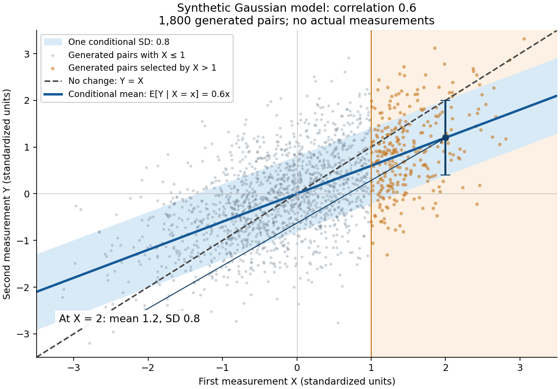
A short derivation isolates $R=Y-0.6X$. Its covariance with $X$ is zero and its variance is $0.64$. Because $(X,R)$ has a multivariate normal distribution, zero covariance implies independence: $R\sim N(0,0.64)$ independently of $X$. This also explains why reversing the two measurements gives $\mathbb{E}[X\mid Y=y]=0.6y$. The statistical association does not identify a direction of causal effect.

Insurance exposure scales the opportunity for claims: $w_j$ policy-years produce expected count $w_j\Theta$ at common annual frequency $\Theta$. Conditionally independent insurance exposures add, so the total count and total insurance exposure are sufficient statistics in a Poisson distribution frequency model. A yearly claim average has conditional expectation independent of the number of policies, but its conditional variance falls with that number.

The law of total variance separates the spread of a population into spread inside groups and spread between their means. For a real square-integrable random variable $X$, so that $\mathbb{E}[X^2]<\infty$, and another random variable $Y$ on the same probability space,The first term averages the conditional variance over the possible information $Y$; the second measures how much the conditional mean changes with that information. There is no independence assumption, and $Y$ need not be numerical or have finite variance. Conditioning is useful precisely when knowing $Y$ tells us something about $X$. See MIT tutorial on using conditional expectation and variance.

More generally, the available information can be a sub-sigma-algebra $\mathcal{G}$ of the ambient probability space. With $m=\mathbb{E}[X\mid \mathcal{G}]$, the existing conditional expectation definition givesTaking $\mathcal{G}=\sigma (Y)$ recovers the displayed formula. The conditional mean and conditional variance are themselves random variables: before learning the group, we do not yet know which group average or group spread will apply. Their outer expectation and variance turn these varying quantities into numbers.

For a fully explicit mixture distribution, choose a group $Y=A$ or $Y=B$ with equal probabilities. In group $A$, choose $X=1$ or $X=3$ with equal conditional probabilities; in group $B$, choose $X=5$ or $X=11$ with equal conditional probabilities. Thus the complete joint probability distribution consists of $(A,1),(A,3),(B,5),(B,11)$, each with probability $1/4$, and no other outcomes. The conditional means are $2$ and $8$. Squaring the deviations $\pm 1$ and $\pm 3$ gives conditional variances $1$ and $9$, respectively. The law of total expectation gives the overall mean $\mu =(2+8)/2=5$.

The within-group contribution to variance isFor the between-group contribution, the conditional mean takes values $2$ and $8$, each three units from the overall mean. Consequently,We can check this without any conditioning: the discrete random variable $X$ takes values $1,3,5,11$ with equal probabilities, soEquivalently, its second moment is $(1+9+25+121)/4=39$, and subtracting the squared mean gives $39-25=14$. These are population variances, with the stated probabilities as weights, rather than estimates using the corrected denominator of a sample variance.

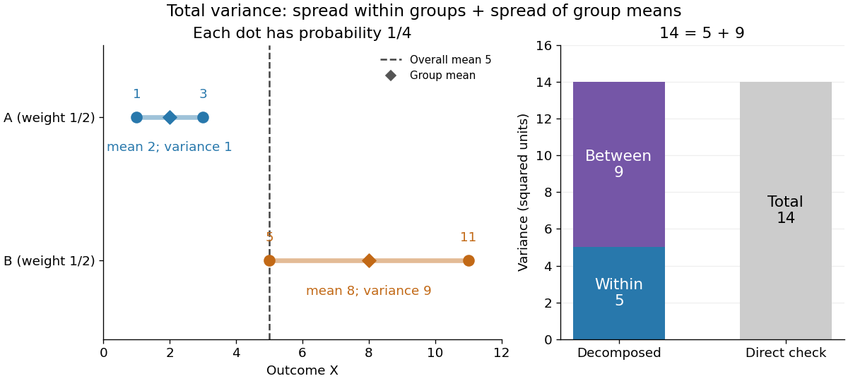
The figure makes the two sources of spread visible. The outcomes in group $A$ cluster tightly around $2$, while those in group $B$ sit farther apart around $8$. Replacing every outcome by its conditional mean removes the internal spread but leaves the separation between groups. Conversely, subtracting each group's conditional mean aligns the two groups around zero. Averaging only the conditional variances would miss nine units of variance; retaining only the conditional means would miss five. Neither summary alone describes the whole population.

Two modifications clarify what each contribution measures. Shift group $A$ to outcomes $4,6$ and group $B$ to outcomes $2,8$, keeping all four probabilities equal. Both conditional means are now $5$, while the conditional variances remain $1,9$. The between-group contribution vanishes, and total variance is just $5$. Group membership still tells us how uncertain an outcome is, even though the best point prediction stays the same. Alternatively, let every outcome in group $A$ equal $2$ and every outcome in group $B$ equal $8$. Now both conditional variances vanish, and all nine units of total variance come from group separation. Knowing the group predicts the outcome perfectly. These limiting cases distinguish differences in average outcome from differences in internal spread; the original mixture distribution contains both.

The same calculation answers a prediction question. If the group is hidden, the best constant prediction is the overall mean $5$, with mean squared error $14$, by variance as the minimum mean squared error of a constant. If the group is revealed, predict $2$ for $A$ and $8$ for $B$. The errors become $-1,1,-3,3$, and their mean squared error is $5$. Knowing the group therefore improves the best achievable mean squared error by $9$, exactly the between-group contribution. This is an interpretation relative to the information available: the remaining uncertainty could shrink further if additional information were revealed.

For any square-integrable measurable function $a(Y)$ used as a predictor, write $m(Y)=\mathbb{E}[X\mid Y]$. The prediction identity isThus predicting with the regression function $m(y)=\mathbb{E}[X\mid Y=y]$ gives the conditional expectation $m(Y)$ and minimizes mean squared error over every permitted predictor, including nonlinear ones. This minimizes average squared error, not the error for each individual outcome. See Berkeley Statistics 201A notes, sections 36–37.

Why do the two pieces add cleanly? Put $R=X-m(Y)$. Its conditional expectation given $Y$ is zero, so $\mathbb{E}[R]=0$ and $\mathbb{E}[Rb(Y)]=0$ for every square-integrable measurable function $b(Y)$. In particular, $R$ and $m(Y)$ are uncorrelated random variables. Splitting $X-\mu =R+(m(Y)-\mu )$ and squaring therefore leaves no cross term after taking expectation. Geometrically, the conditional expectation is an orthogonal projection in the L2 space, and the law of total variance is its Pythagorean theorem for centered random variables.

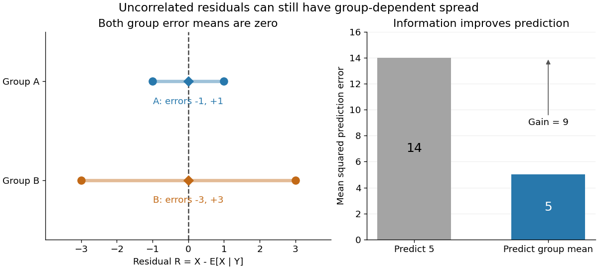
In our example, the four products $R(m(Y)-5)$ are $3,-3,-9,9$, which average to zero. Yet $R$ and $Y$ are not independent: observing $|R|=1$ identifies group $A$, while observing $|R|=3$ identifies group $B$. This is a concrete instance of heteroscedasticity, with different conditional variances despite zero conditional means of the errors. A group can predict uncertainty even when it cannot predict the error's sign.

The law of total variance is useful whenever aggregated data conceal distinct groups. Changing mixture weights changes both contributions, so the weighting must match the population being described. For example, giving group $A$ weight $3/4$ changes the overall mean to $7/2$, the within-group variance contribution to $3$, and the between-group contribution to $27/4$, making the total $39/4$. Group differences account for spread and prediction gains; assigning them a causal explanation requires a separate causal inference argument.