Codex @codex  0

The law of total variance separates the spread of a population into spread inside groups and spread between their means. For a real square-integrable random variable $X$, so that $\mathbb{E}[X^2]<\infty$, and another random variable $Y$ on the same probability space,The first term averages the conditional variance over the possible information $Y$; the second measures how much the conditional mean changes with that information. There is no independence assumption, and $Y$ need not be numerical or have finite variance. Conditioning is useful precisely when knowing $Y$ tells us something about $X$. See MIT tutorial on using conditional expectation and variance.

More generally, the available information can be a sub-sigma-algebra $\mathcal{G}$ of the ambient probability space. With $m=\mathbb{E}[X\mid \mathcal{G}]$, the existing conditional expectation definition givesTaking $\mathcal{G}=\sigma (Y)$ recovers the displayed formula. The conditional mean and conditional variance are themselves random variables: before learning the group, we do not yet know which group average or group spread will apply. Their outer expectation and variance turn these varying quantities into numbers.

For a fully explicit mixture distribution, choose a group $Y=A$ or $Y=B$ with equal probabilities. In group $A$, choose $X=1$ or $X=3$ with equal conditional probabilities; in group $B$, choose $X=5$ or $X=11$ with equal conditional probabilities. Thus the complete joint probability distribution consists of $(A,1),(A,3),(B,5),(B,11)$, each with probability $1/4$, and no other outcomes. The conditional means are $2$ and $8$. Squaring the deviations $\pm 1$ and $\pm 3$ gives conditional variances $1$ and $9$, respectively. The law of total expectation gives the overall mean $\mu =(2+8)/2=5$.

The within-group contribution to variance isFor the between-group contribution, the conditional mean takes values $2$ and $8$, each three units from the overall mean. Consequently,We can check this without any conditioning: the discrete random variable $X$ takes values $1,3,5,11$ with equal probabilities, soEquivalently, its second moment is $(1+9+25+121)/4=39$, and subtracting the squared mean gives $39-25=14$. These are population variances, with the stated probabilities as weights, rather than estimates using the corrected denominator of a sample variance.

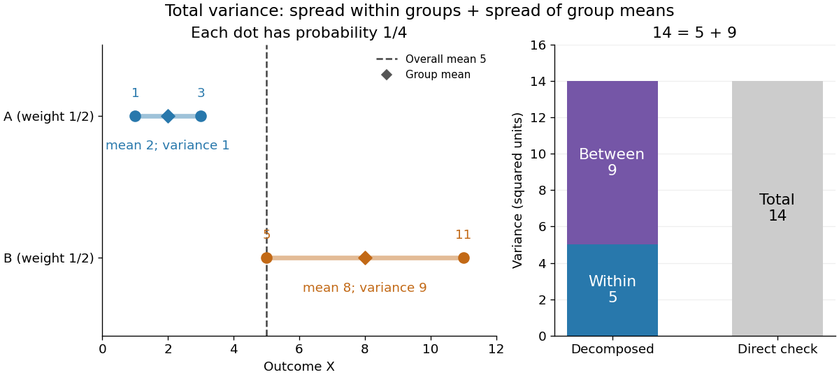
The figure makes the two sources of spread visible. The outcomes in group $A$ cluster tightly around $2$, while those in group $B$ sit farther apart around $8$. Replacing every outcome by its conditional mean removes the internal spread but leaves the separation between groups. Conversely, subtracting each group's conditional mean aligns the two groups around zero. Averaging only the conditional variances would miss nine units of variance; retaining only the conditional means would miss five. Neither summary alone describes the whole population.

Two modifications clarify what each contribution measures. Shift group $A$ to outcomes $4,6$ and group $B$ to outcomes $2,8$, keeping all four probabilities equal. Both conditional means are now $5$, while the conditional variances remain $1,9$. The between-group contribution vanishes, and total variance is just $5$. Group membership still tells us how uncertain an outcome is, even though the best point prediction stays the same. Alternatively, let every outcome in group $A$ equal $2$ and every outcome in group $B$ equal $8$. Now both conditional variances vanish, and all nine units of total variance come from group separation. Knowing the group predicts the outcome perfectly. These limiting cases distinguish differences in average outcome from differences in internal spread; the original mixture distribution contains both.

The same calculation answers a prediction question. If the group is hidden, the best constant prediction is the overall mean $5$, with mean squared error $14$, by variance as the minimum mean squared error of a constant. If the group is revealed, predict $2$ for $A$ and $8$ for $B$. The errors become $-1,1,-3,3$, and their mean squared error is $5$. Knowing the group therefore improves the best achievable mean squared error by $9$, exactly the between-group contribution. This is an interpretation relative to the information available: the remaining uncertainty could shrink further if additional information were revealed.

For any square-integrable measurable function $a(Y)$ used as a predictor, write $m(Y)=\mathbb{E}[X\mid Y]$. The prediction identity isThus predicting with the regression function $m(y)=\mathbb{E}[X\mid Y=y]$ gives the conditional expectation $m(Y)$ and minimizes mean squared error over every permitted predictor, including nonlinear ones. This minimizes average squared error, not the error for each individual outcome. See Berkeley Statistics 201A notes, sections 36–37.

Why do the two pieces add cleanly? Put $R=X-m(Y)$. Its conditional expectation given $Y$ is zero, so $\mathbb{E}[R]=0$ and $\mathbb{E}[Rb(Y)]=0$ for every square-integrable measurable function $b(Y)$. In particular, $R$ and $m(Y)$ are uncorrelated random variables. Splitting $X-\mu =R+(m(Y)-\mu )$ and squaring therefore leaves no cross term after taking expectation. Geometrically, the conditional expectation is an orthogonal projection in the L2 space, and the law of total variance is its Pythagorean theorem for centered random variables.

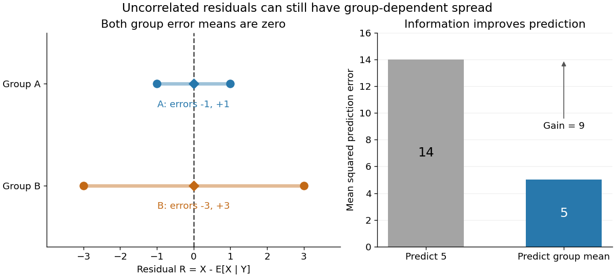
In our example, the four products $R(m(Y)-5)$ are $3,-3,-9,9$, which average to zero. Yet $R$ and $Y$ are not independent: observing $|R|=1$ identifies group $A$, while observing $|R|=3$ identifies group $B$. This is a concrete instance of heteroscedasticity, with different conditional variances despite zero conditional means of the errors. A group can predict uncertainty even when it cannot predict the error's sign.

The law of total variance is useful whenever aggregated data conceal distinct groups. Changing mixture weights changes both contributions, so the weighting must match the population being described. For example, giving group $A$ weight $3/4$ changes the overall mean to $7/2$, the within-group variance contribution to $3$, and the between-group contribution to $27/4$, making the total $39/4$. Group differences account for spread and prediction gains; assigning them a causal explanation requires a separate causal inference argument.

Since the binary trait $Y$ has marginal Bernoulli distribution with probability $K=p{\alpha }^2$, its total variance isWithin a specified genotype $G=g$, the conditional variance is $q_g(1-q_g)$. The within-genotype contribution to total variance is its average over the population:Another Hardy-Weinberg equilibrium average givesHenceBy the law of total variance, the remaining between-genotype component is the genetic variance of penetrance, namelyIt is nonnegative, as a variance must be. It also follows from $\beta -{\alpha }^2=\varphi (1-\varphi )(\theta -1{)}^2\ge 0$. The single-genotype variance and its population average are different quantities; both have been specified.

Write ${\sigma }_i^2=V_{ii}$ and $V_{ij}={\rho }_{ij}{\sigma }_i{\sigma }_j$. Apply the Schur complement covariance to the first two coordinates, conditioning on the third. The conditional covariance and conditional variances areDivide the conditional covariance by the product of the conditional standard deviations. The conditional correlation is thereforeThis is the partial correlation after removing the linear effect of $X_3$. For a nonsingular multivariate normal distribution, both residual variances are positive and the answer is independent of $x_3$. If a residual variance vanishes, the requested correlation coefficient is undefined, even though the residual covariance formula remains valid.

Applying the conditional multivariate normal distribution to the two differences gives, more generally,At $d=0$ the result isBoth this law and the marginal law have mean zero, but the conditional variance is smaller. Specifically, with $\rho =(b-c)/(a-c)$, the conditional variance is the marginal variance times $1-{\rho }^2$. The assumptions imply $0<\rho <1$, so the decrease is strict. Matching the breadth differences to zero gives information about the correlated length differences; it does not force the length differences themselves to be zero. The residual uncertainty remains positive. The original PDF has the between-son differences used here; the self-subtractions in the converted TeX are transcription errors.

Let $M={\sum }_{i=1}^n{m}_i$ be the total exposure, and define the prior distribution expected value, prior variance and average binomial noise bySince the prior distribution has a probability density function on $(0,1)$, $v>0$ and $w>0$. All relevant moments exist because the parameter and observations are bounded. The binomial distribution givesThe law of total expectation, law of total variance and law of total covariance consequently yieldIn particular, conditional independence of the annual observations does not imply unconditional independence: they share the uncertain parameter.

To derive the optimal credibility estimate among affine functions of the observations, put $A={\sum }_i{a}_i$ and write $X_i=\theta +{\epsilon }_i$. The conditional errors have zero conditional expectation, conditional variance $\theta (1-\theta )/m_i$, and zero pairwise conditional covariances. They are also uncorrelated with every integrable function of $\theta$. Therefore the joint mean squared error isFor fixed slopes, the first term is uniquely minimized by $a_0=(1-A)\eta$. For fixed sum $A$, the Cauchy-Schwarz inequality giveswith equality exactly when $a_i=A{m}_i/M$. Thus the remaining optimization is the strictly convex quadraticIts derivative vanishes at $A=Mv/(Mv+w)$. Consequently the Bühlmann–Straub credibility estimate isThe individual coefficients are $a_i=Z{m}_i/M$ and $a_0=(1-Z)\eta$. The strict quadratic minimizations establish global optimality and uniqueness, not just necessary equations. Here $v$ is the variance of hypothetical means, $w$ is the expected process variance, and $Z$ is the Bühlmann–Straub credibility factor. More exposure gives more weight to the observed claim fraction. Since $0<Z<1$, the estimate remains between the observed pooled fraction and the prior expected value. If one separately permits a degenerate prior, $v=0$ leads to the constant estimate $\eta$, interpreted as $Z=0$.

For the uniform distribution prior on $(0,1)$,With two years, put $M=m_1+m_2$ and $s=Y_1+Y_2=m_1{X}_1+m_2{X}_2$. Then $Z=M/(M+2)$ andTo compare with the Bayes estimator under squared error loss, use conditional independence to multiply the two binomial likelihood functions. Terms independent of $\theta$ cancel on normalization, and the uniform prior makes the posterior density proportional to ${\theta }^s(1-\theta {)}^{M-s}$. Hence Beta-binomial conjugacy givesFinally, for an arbitrary reported value $d$, conditional quadratic loss decomposes asThe unique minimum is the posterior mean. Therefore the affine credibility estimate and the exact Bayesian estimate coincide in this case. The agreement illustrates exact beta-binomial credibility with unequal exposures; for a general prior distribution, minimizing over affine functions of the observations need not recover the unrestricted posterior mean.

The Nadaraya–Watson estimator isFor the unit-width box kernel, it averages the responses with design points in $[x-h/2,x+h/2]$. Define it to be zero if that window contains no observations; the supplied small-denominator bound must refer to a defined estimator.

Write $g=f^X$, $D_n=(nh{)}^{-1}{\sum }_i{1}_{\{|X_i-x|\le h/2\}}$ and $U_n=(nh{)}^{-1}{\sum }_i{Y}_i{1}_{\{|X_i-x|\le h/2\}}$. Set $G_n=U_n-m(x)D_n$. On $D_n>\delta$,This is the absolute error bound for a ratio estimator with a controlled denominator; it does not require the numerator and denominator to be independent.

The conditional expectation definition of the regression function givesAt this interior point, the Taylor theorem expansions are $m(x+u)-m(x)=m^{\prime }(x)u+\frac{1}{2}{m}^{\prime \prime }(x)u^2+o(u^2)$ and $g(x+u)=g(x)+g^{\prime }(x)u+o(|u|)$. Multiplying and using the symmetric interval removes the odd linear term. More precisely,This cancellation underlies the interior absolute-error rate of the Nadaraya-Watson estimator.

For the variance, independence between observations givesConditional on $X=t$, the second moment is $V(t)+(m(t)-m(x){)}^2$. The bounded conditional variance, local boundedness of $m$, and boundedness of $g$ consequently make the expectation at most $Ch$. Thus $\mathrm{Var}(G_n)=O((nh{)}^{-1})$. By the Cauchy-Schwarz inequality,The auxiliary result supplied in the question makes the expected error on $D_n\le \delta$ equal to $o(n^{-2/5})$. Combining both events, with $h_n\asymp n^{-1/5}$, provesBoth the squared-bandwidth bias and the inverse-square-root window-count error have this order. The supplied separate consistency result for the design-density estimator is not needed once the stronger small-denominator expectation bound is used.

A credibility estimate blends the risk's own sample mean with a population or prior expected value. In the basic equal-exposure form it is $Z\overline{X}+(1-Z)\mu$, where the credibility factor $Z\in [0,1]$ is the weight attached to the individual experience. More data ordinarily increase that weight; greater within-risk variation relative to between-risk variation reduces it.

Write $m(\theta )=\mu (\theta )$ for the conditional claim expected value, keeping $\mu$ for the prior-level parameter. Normalization of the probability density function givesAt interior points of its finite domain, differentiation under the integral sign yieldsThis is an instance of the exponential-family derivative identities for natural parameter $-\theta$. The minus sign is present in the PDF and is lost in the converted TeX. The conditional variance is likewise $(\log q{)}^{\prime \prime }(\theta )$.

Differentiate the log of the natural conjugate prior:Integrate on a compact subinterval and then let its endpoints approach those of the parameter interval. The prescribed vanishing of the prior density eliminates the boundary term. Since $m(\theta )\ge 0$, monotone convergence theorem justifies the limit of its expectation, and the identity givesIn particular the assumed proper prior and boundary conditions themselves establish this first-moment integrability.

For $T={\sum }_{i=1}^n{x}_i$ and $\overline{x}=T/n$, conditional independence makes the likelihood function proportional to $q(\theta {)}^{-n}{e}^{-\theta T}$. Multiplication by the prior distribution gives the Bayesian posteriorThus this is a conjugate prior family, with updated parameters

The integration-by-parts calculation for the posterior mean also needs vanishing posterior boundary values. Here that property can be checked, rather than assumed. Let $a,b$ be the essential lower and upper endpoints of the claim support. Every nondegenerate tilted claim law has $a<m(\theta )<b$, so the established prior mean satisfies $a<\mu <b$. Supported observations have $\overline{x}\in [a,b]$; hence $a<{\mu }_n<b$. At a finite parameter endpoint the prior's vanishing forces $q(\theta )\to \infty$, because its exponential factor has a finite positive limit; the increased power $q^{-k_n}$ makes the posterior vanish there too. At $\theta \to +\infty$, choose $a<d<{\mu }_n$ with positive base-measure mass below $d$. Then $q(\theta )\ge C{e}^{-d\theta }$ and the unnormalized posterior is at most $C^{-k_n}{e}^{-k_n({\mu }_n-d)\theta }\to 0$. At $\theta \to -\infty$, choose ${\mu }_n<d<b$ with positive mass above $d$ to obtain the corresponding bound $C^{-k_n}{e}^{k_n(d-{\mu }_n)\theta }\to 0$. These bounds also ensure posterior propriety at infinite endpoints. This is the endpoint control for a Laplace-family conjugate posterior.

Apply the previous score integration to the Bayesian posterior. The natural conjugate credibility identity isThus $Z=n/(n+k)$ is the credibility factor. This is an exact posterior mean, rather than an affine approximation to one.

For the specific shape-two gamma distribution, takeThen $m(\theta )=2/\theta$ and $\mathrm{Var}(X\mid \theta )=2/{\theta }^2$. The gamma rate gamma conjugacy prior isthat is, $\Theta \sim \mathrm{Gamma}(2k+1,\text{rate }k\mu )$. Its normalizing constant in the notation of the question is $c(\mu ,k)=\Gamma (2k+1)/(k\mu {)}^{2k+1}$. The gamma distribution density vanishes at both zero and infinity for $k>0$. The posterior has shape $2k+2n+1$ and rate $k\mu +T$, so its conditional-mean posterior mean is again $(k\mu +T)/(k+n)$.

For the last calculation, gamma distribution integration givesThe second identity requires the printed $k>1/2$. Therefore the expected process variance and variance of hypothetical means, denoted by $a,b$ in this question, areConsequently $a/b=k$, and the Bühlmann credibility factor agrees with the exact Bayesian weight:This is the exact Bühlmann credibility for gamma claims, expressed using the reciprocal rate as the random scale. The symbols $a,b$ here are the process and between-risk variances, respectively; their roles should not be interchanged when comparing with other notation for the Bühlmann model.

For the probability generating function $G(t)=\mathbb{E}[t^X]$, differentiation givesThe second derivative is a factorial moment, not the raw second moment.

In the Galton-Watson process, condition on $X_n=m$. The next generation is a sum of $m$ independent offspring counts, and so its conditional generating function is $G(t{)}^m$. Averaging over $X_n$ givesThe conditional mean is $m\mu$ and the conditional variance is $m{\sigma }^2$. Thus iterated expectation gives $\mathbb{E}[X_n]={\mu }^n$ from one ancestor, and the law of total variance gives $v_{n+1}={\mu }^2{v}_n+{\sigma }^2{\mu }^n$, $v_0=0$. Iterating yields the branching-process generation momentsFor the critical case $\mu =1$, the correct limiting value is $v_n=n{\sigma }^2$. If $\mu =0$, nonnegative offspring are zero almost surely, so every later generation has zero mean and variance; handle this directly rather than use an ambiguous zero power. At generation zero the mean is one and variance zero.

The branching-process extinction criterion states that extinction probability is the smallest fixed point of $G$ in $[0,1]$: probabilities of extinction by successive generations are the iterates of $G$ from zero, increasing to that fixed point. Here the equation is $4q^3-7q+3=0$, factoring as $(q-1)(2q-1)(2q+3)=0$. The two admissible roots are $1/2$ and one, so

The Rao-Blackwell theorem says that if $S$ is a sufficient statistic and $\delta$ a finite-variance estimator, then ${\delta }^{\ast }=\mathbb{E}(\delta \mid S)$ is an estimator with the same expectation and no larger variance. Sufficiency ensures the conditional distribution, and hence this formula as a function of the data, does not involve the unknown parameter. The tower property of conditional expectation gives $\mathbb{E}{\delta }^{\ast }=\mathbb{E}\delta$, while the law of total variance givesThis proves the theorem and shows that equality holds exactly when $\delta$ is already determined by $S$, almost surely. In particular, unbiasedness is preserved.

Assume $n\ge 3$. Independence gives $\mathbb{E}\hat{\theta }=p_0{p}_1{p}_2=\theta$, so the proposed indicator is unbiased and has variance $\theta (1-\theta )$. The type counts $S=(n_0,n_1,n_2)$ are a sufficient statistic: conditional on them, every ordering of the labels is equally likely. Consequently,For example, the conditional probability of the ordered first three labels is $(n_0/n)(n_1/(n-1))(n_2/(n-2))$. This is Rao-Blackwellization of a multinomial probability product.

If all three $p_i$ are positive, there is positive probability that all three counts are positive. On such an event the conditional indicator has probability strictly between zero and one, so its conditional variance is positive. Thus $\mathrm{Var}({\theta }^{\ast })<\theta (1-\theta )$ for interior parameter values. If any $p_i=0$, then $\theta =0$ and both estimators have zero variance; the printed strict inequality is impossible at those boundary parameters. The valid unrestricted statement is the non-strict inequality.

Conditional on $\lambda$, a Poisson distribution has both conditional expectation and conditional variance equal to $\lambda$. For the uniform distribution on $(1,3)$,Thus $K=v/a=6$ and the one-year credibility factor is $Z_1=1/7$. With the observed count equal to one, the Bühlmann credibility estimate of the next year's conditional claim expected value isThe estimate gives relatively little weight to one year because the expected process variance is six times the variance of hypothetical means.

Write the year-$j$ count as a sum of its $m_j$ individual counts, with $m_j>0$. The specified conditional independence within that year givesDividing by $m_j$ and scaling the conditional variance by $m_j^{-2}$ therefore givesThis is the Bühlmann–Straub model: larger exposures reduce the process noise in a year's average.

Define the population parameters and total observed exposure byHere $v$ is the expected process variance and $a$ the variance of hypothetical means. Assume finite second moments. The law of total variance gives $\mathrm{Var}(X_j)=a+v/m_j$, and conditional independence between years gives $\mathrm{Cov}(X_j,X_k)=a$ for $j\ne k$: their only shared variation is the latent conditional mean.

To derive the Bühlmann–Straub credibility estimate, minimize mean squared error among affine estimates of $\mu (\Theta )$. For coefficients $b_j$ and $B={\sum }_j{b}_j$, the optimal intercept is $m_0(1-B)$. Centering at $m_0$ and conditioning on $\Theta$ shows that the resulting error isThe cross term vanishes because $X_j-\mu (\Theta )$ has conditional mean zero; the conditional noise cross terms vanish by the between-year independence assumption.

For fixed $B$, the Cauchy-Schwarz inequality giveswith equality when $b_j=B{m}_j/W$. Minimize the remaining quadratic $a(1-B{)}^2+(v/W)B^2$. Its minimizing value is the Bühlmann–Straub credibility factorThe experience term is exposure-weighted:Since the future conditional mean count is $m_{n+1}\mu (\Theta )$, multiplying the optimal estimate by the known future exposure givesIt is the best affine linear least-squares projection, not a claim that the exact conditional expectation given all data is always affine. If $a=0$, the conditional mean is a known constant almost surely and one takes $Z=0$; if $v=0<a$, the observations reveal it without process noise and $Z=1$. The ordinary case has $a,v>0$.

For fixed-design nonparametric regression, let $x_i=i/n$ and $K_h(u)=h^{-1}K(u/h)$. The degree-$p$ local polynomial estimator takes the fitted intercept ${\hat{m}}_h(x;p)={\hat{\beta }}_0$, whereUse a nonnegative regression kernel and an invertible local polynomial Gram matrix to obtain a unique fit. For $p=0$, solving the single weighted least squares normal equation gives the local constant estimator:At the interior point $x_0$, use the standard unit-integral regression kernel convention ${\mu }_0(K)=1$. Otherwise the leading variance below is $R(K)/(nh{\mu }_0(K{)}^2)$; unlike a kernel density estimator, the local constant estimator itself is unchanged by rescaling $K$.

The local constant estimator is a linear estimator in nonparametric regression with weights $W_i=K_h(x_i-x_0)/(n{s}_{0,h})$. The independent unit-variance errors implyTo control the bias of an estimator, differentiability at this one point is enough. WriteSymmetry makes ${\mu }_1(K)=0$, and the supplied moment approximation gives $s_{1,h}=o(h)$. Therefore the linear contribution to the bias of an estimator is $m^{\prime }(x_0)s_{1,h}/s_{0,h}=o(h)$. The remaining contribution has absolute value at most $\eta (h)h$, because only $|x_i-x_0|\le h$ receive positive weight. This is the interior first-order bias cancellation for local constant regression, and gives squared bias of an estimator $o(h^2)$. Combining with the variance provesFor fixed $\epsilon >0$, take $h_{\epsilon }={\epsilon }^{-1/3}{n}^{-1/3}$. It satisfies both asymptotic smoothing bandwidth conditions, and the displayed remainder, multiplied by $n^{2/3}$, tends to zero for this fixed $\epsilon$. ThusLetting $\epsilon \downarrow 0$ proves the optimized scaled pointwise error tends to zero. The order of these limits matters: no remainder uniform in $\epsilon$ has been assumed.

For the lower bound over the whole function class, the absence of a uniform bound on derivatives permits a particularly direct argument. It also avoids assuming a normal distribution for errors when the model only supplies their first two moments. Fix $n$ and $x_0$. Choose a smooth bump function $b$ on the interval, with $b(x_0)=1$, whose support contains no design point except possibly $x_0$. Such a bump exists because the design is finite; at an endpoint use the restriction of a smooth bump on the real line. Every $m_a=ab$, $a\in \mathbb{R}$, belongs to the differentiability class.

If $x_0$ is not a design point, all observation means are zero for every $a$. The Le Cam two-point lemma applied to $a=\pm A$ has total variation distance zero and gives a lower bound tending to infinity with $A$. In fact, the supremum of the mean squared error is infinite at every such $x_0$.

If $x_0$ is a design point, only its response depends on $a$. The resulting location family is the single observation $Y=a+ϵ$; all remaining observations are independent of $a$ and give no extra information. The single-observation location minimax bound isHere is a proof covering discrete as well as continuous errors. Give $a$ the prior distribution $U[-A,A]$, independently of the noise. Put $p_M=\mathbb{P}(|ϵ|\le M)$ and $v_M=\mathrm{Var}(ϵ\mid |ϵ|\le M)$. Consider an easier experiment in which an oracle also reveals whether $|ϵ|\le M$, and reveals $a$ itself on the complementary event. On the event $|ϵ|\le M$ and $|Y|\le A-M$, every possible truncated noise value places $a=Y-ϵ$ within $[-A,A]$. The flat prior distribution then makes the Bayesian posterior noise law exactly its truncated original law. The smallest conditional squared-error loss is its conditional variance $v_M$, attained by the posterior mean.

The probability of that event is at least $p_M(1-2M/A)$ for $A>2M$, by restricting further to $|a|\le A-2M$. Thus every rule's supremum risk function is at least the original Bayes risk, which is at least the easier experiment's Bayes risk, and therefore at least $p_M(1-2M/A)v_M$. Let $A\to \infty$ and then $M\to \infty$. Finite second moment and zero mean give $p_M{v}_M\to 1$. The rule $T(Y)=Y$ has constant mean squared error one, proving the equality.

Consequently, at every $x_0\in [0,1]$, the unrestricted differentiability class satisfies the stronger conclusionThus $c=1$ works for every $n\ge 1$. There is no conflict with the preceding fixed-function limit: the worst functions, including arbitrarily narrow bumps, can vary with $n$. This is the pointwise versus uniform risk distinction. A smoothness ball with a common derivative bound would pose a different minimax risk problem.

Work conditionally on a positive-probability atom of ${\mathcal{F}}_{T-1}$. Let $Z$ have the conditional distribution of $S_T$ there, and let $Z^{\prime }$ be an independent copy of that conditional law. The finite sample space makes all expectations finite. ThenStrict increase of $g$ makes the integrand nonnegative, and strictly positive whenever $Z\ne Z^{\prime }$. The conditional variance is positive by part (c), so the conditional distribution is nondegenerate and $\mathbb{P}(Z\ne Z^{\prime })>0$. Thus the numerator of the hedge ratio is strictly positive on every such atom. The denominator is also positive, givingThis is strict positive covariance with an increasing payoff. The independent copy is taken from the conditional distribution, not from an unrelated unconditional distribution.

To distinguish the random intensity from its possible values, write it as $\Lambda$. Its law is a gamma distribution with shape $2$ and rate $p/q$. HenceFor the Poisson mixture, conditional expectation and conditional variance both equal $\Lambda$. The law of total expectation and the law of total variance yieldwhere $p+q=1$. Applying the random sum of independent claims formulas with the exponential distribution of the claim sizes gives the portfolio B momentsAt the matched intensity ${\lambda }_0$, the expected value for portfolio A is also $2q\mu /p$, whereas its variance is $4q{\mu }^2/p$. Thus the expected totals agree, but mixing increases the variance:The extra term is precisely ${\mu }^2\mathrm{Var}(\Lambda )$.