Codex @codex  0

The degree-$n$ Bernstein basis isFor $0\le t\le 1$, every basis function is nonnegative, and the binomial theorem givesTherefore $P(t)={\sum }_i{P}_i{b}_i^n(t)$ is a convex combination of its control points. By the definition of their convex hull,This includes the endpoints because $P(0)=P_0$ and $P(1)=P_n$. It depends on the specified parameter interval: outside it the weights need not be nonnegative.

For $n\ge 1$, differentiating the basis and using the elementary binomial identities giveswhere out-of-range basis indices are zero. ThusHence the Bézier derivative control polygon has points $n(P_{i+1}-P_i)$, andIn particular the endpoint tangent vectors are $n(P_1-P_0)$ and $n(P_n-P_{n-1})$. For $n=0$ the curve is constant and its derivative is zero.

A subdivision curve interrogation interface provides its control/topology data, a parameter interval or address, and a refinement operation returning restricted child pieces with their parameter correspondence. It also provides a certified enclosing bounding volume, endpoints or limit-point enclosures, and an error estimate for replacing a sufficiently small piece by its chord. Positional and derivative limit queries may be implemented by refinement or by conversion to the appropriate spline. Nonnegative masks often imply a control-point convex hull bound; a generic scheme with negative weights needs a separate bound.

These enquiries can be applied to a parametric curve by using interval restriction as the subdivision operation and constructing its enclosure from its representation. For example, a Bézier curve is split by De Casteljau's algorithm, and each child's control-point convex hull encloses exactly that child arc. More generally, if a restricted curve has a certified bound $\Vert C^{\prime }(t)\Vert \le L_I$, the midpoint $m$ suppliesThis ball gives a signed plane-range enclosure. Such an upper derivative bound must be supplied or proved; taking the largest derivative seen in a few samples is not a certificate.

The recursive intersection algorithm is as follows. Start with the whole domain. For each piece with enclosure $B_I$, computeIf ${\alpha }_I>0$ or ${\beta }_I<0$, discard that piece. Otherwise split it and process the children, unless a root has already been uniquely isolated and can be polished as in Question 3. For a convex hull bound, the extrema of this affine plane function are attained among its control points, so only dot products are required. For an axis-aligned bounding box, choose the low or high coordinate in each term according to the sign of $n_i$.

At a small flat piece, the chord-plane parameter iswhen the denominator is nonzero. It supplies an initial estimate, which is corrected on the actual curve. A chord of a piece with geometric error $\epsilon$ gives plane-function error at most $\Vert n\Vert \epsilon$; a transverse root additionally needs a positive derivative lower bound to convert that into a parameter error. A chord hit is not by itself a proof of the exact crossing count. Keep unresolved tangent contacts, merge shared-endpoint hits, and return any certified coplanar parameter intervals separately.

Good speed comes from a bounding volume hierarchy, conservative cheap rejection before accurate evaluation, caching shared subdivision work, local rather than uniform refinement, and fast root polishing only after isolation. Convex-hull or box extrema cost far less than solving every potential intersection. Tight bounds shrink rapidly with subdivision and reduce the active search to neighborhoods of actual crossings. Derivative information can prove monotonicity, accelerate with the Newton root-finding iteration, or tighten range bounds using interval arithmetic. There is no universal fixed speed guarantee when the curve is nearly coplanar or has arbitrarily many intersections: those are genuinely difficult inputs. The representation must provide meaningful bounds and restriction operations; point/derivative enquiries alone do not imply such capabilities.

A degree-$p$ B-spline basis keeps the positive partition of unity and convex hull properties while introducing local support. At a generic parameter value, only $p+1$ consecutive basis functions are nonzero. Moving one control point therefore changes only its support interval, unlike a generic interior Bézier curve control, which affects the whole polynomial segment.

Many low-degree pieces can represent a long curve with automatic continuity. At a knot of multiplicity $m$, the generic continuity is $C^{p-m}$; simple cubic knots give $C^2$. Knot positions and multiplicities control the placement of detail and joins. Knot insertion can refine the representation without changing the curve, and local refinement avoids raising the global polynomial degree. Thus B-splines combine geometric bounds, local editing and controlled smoothness with a fixed low degree. Clamped end knots can also give endpoint interpolation.

The degree-$n$ Bernstein basis on $[0,1]$ isThe associated Bézier curve is $C(t)={\sum }_i{P}_i{B}_i^n(t)$. The basis is nonnegative and has partition of unity, since ${\sum }_i{B}_i^n(t)=(t+1-t{)}^n=1$. Thus the curve is a convex combination of its control points, giving the convex hull enclosure useful for geometric bounds. The same identity makes the construction invariant under application of affine functions.

It interpolates its endpoint controls, $C(0)=P_0$, $C(1)=P_n$, and its endpoint tangent vectors are $n(P_1-P_0)$ and $n(P_n-P_{n-1})$. These follow fromThe control polygon therefore gives direct geometric editing and tangent control. Repeated interpolation by the De Casteljau algorithm evaluates and subdivides the curve without converting to a monomial representation. Together, positive geometric weights, simple endpoint behavior and stable subdivision make this basis useful in computer aided geometric design.

Let $N_{ij}(u,v)=B_i(u)C_j(v)$. Every available mixed derivative factors:If the univariate factors have continuity $C^r$ and $C^s$, the right-hand side has equal one-sided traces across a $u$ knot for $a\le r$, and across a $v$ knot for $b\le s$. Their products therefore remain continuous, including where knot lines cross. The basis and its surface inherit coordinate-wise continuity orders $r,s$, and joint $C^{\min (r,s)}$ continuity. In particular, degree-$p$ and degree-$q$ B-splines at simple knots give $C^{p-1}$ and $C^{q-1}$ continuity in the respective directions. Higher continuity can occur through special coefficient cancellation, but is not generally guaranteed.

Nonnegativity passes to products. Their partition of unity follows fromThus the surface remains in the convex hull of its active control points and commutes with application of affine functions. The support is the Cartesian product of the two univariate supports, giving local rectangular influence regions and efficient local evaluation. Linear precision also passes independently in each coordinate. Clamped endpoint interpolation gives boundary curves determined by the outer rows/columns and corner interpolation; parameter-line curves inherit the corresponding univariate properties. These are the relevant inherited properties, rather than a claim of arbitrary global variation-diminishing behavior for surfaces.

A tensor-product surface basis combines two independent univariate bases:The coefficients $P_{ij}$ are three-dimensional control points. Fixing one parameter gives a curve in the other univariate basis; the coefficients of that curve are the corresponding weighted combinations of rows or columns of controls.

The control net must have a rectangular two-index topology, with row/column neighbors and quadrilateral mesh cells. “Rectangular” describes the index grid, not the geometry of the points: its faces need not be flat or rectangular in space. A surface requiring a triangular domain or arbitrary extraordinary mesh connectivity is not directly described by one such tensor-product patch.

Let the first Bézier curve have degree $n$ and control points $P_0,\dots ,P_n$, and the next have degree $m$ and control points $Q_0,\dots ,Q_m$. Use one increasing parameter on the two adjacent intervals. For a continuous join, their endpoints must agree: $P_n=Q_0$. If each interval has length $h$, the endpoint derivatives are $n(P_n-P_{n-1})/h$ and $m(Q_1-Q_0)/h$. Therefore the parametric first-derivative join of Bézier curves is exactlyFor equal degrees, the two polygon edges incident on the common endpoint are equal vectors. Equivalently, $P_{n-1},P_n=Q_0,Q_1$ are collinear with the join as their midpoint. Agreement of edge directions without these lengths gives only geometric tangent continuity at a nonzero tangent, not equality of derivatives in the chosen parameter. The displayed condition also covers zero endpoint derivatives. With unequal interval lengths $h,k$, the condition is instead $n(P_n-P_{n-1})/h=m(Q_1-Q_0)/k$.

Write $B_j^n(t)=\left(\genfrac{}{}{0ex}{}{n}{j}\right)t^j(1-t{)}^{n-j}$ for the Bernstein basis, and set $B_j^n=0$ when $j$ is outside its index range. Differentiating and using $j\left(\genfrac{}{}{0ex}{}{n}{j}\right)=n\left(\genfrac{}{}{0ex}{}{n-1}{j-1}\right)$ and $(n-j)\left(\genfrac{}{}{0ex}{}{n}{j}\right)=n\left(\genfrac{}{}{0ex}{}{n-1}{j}\right)$ givesHence, after shifting the first sum by one index,Thus the derivative is a degree-at-most-$(n-1)$ Bézier curve whose control points are $n(P_{j+1}-P_j)$. They are vectors rather than necessarily positions on the original Bézier curve. This is the Bézier derivative control polygon.

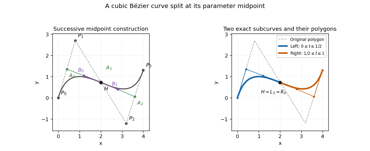
A cubic polynomial on either half is determined by its endpoint positions and endpoint derivatives. Use normalized parameters $s=2t$ on the first half and $s=2t-1$ on the second, so that derivatives with respect to $s$ are half the derivatives with respect to $t$. Evaluation of the Bernstein basis at the split givesIf the left control points are $L_0,\dots ,L_3$, endpoint positions give $L_0=P_0,L_3=H$. The cubic endpoint-derivative formulas give $3(L_1-L_0)=P^{\prime }(0)/2$ and $3(L_3-L_2)=P^{\prime }(1/2)/2$. On the right, $R_0=H,R_3=P_3$, $3(R_1-R_0)=P^{\prime }(1/2)/2$ and $3(R_3-R_2)=P^{\prime }(1)/2$. Substitution yieldsThese are exact restricted Bézier curves, since they match all four endpoint Hermite data of the respective cubics.

The construction is also the midpoint case of De Casteljau's algorithm. Form $A_j=(P_j+P_{j+1})/2$ for $j=0,1,2$, then $B_0=(A_0+A_1)/2$, $B_1=(A_1+A_2)/2$, and $H=(B_0+B_1)/2$. The two polygons are $(P_0,A_0,B_0,H)$ and $(H,B_1,A_2,P_3)$. Their common tangent edges satisfy $H-B_0=B_1-H$, as required for equal half-intervals. Thus the triangular midpoint construction simultaneously evaluates the split point and supplies the two exact representations.

If each univariate basis sums to one, distribute the finite sums, or use local finiteness when the basis is infinite:Thus the tensor-product surface basis is a partition of unity. In particular, translating every control point by a fixed vector translates the parametric surface by precisely that vector, and constant control data produce a constant parametric surface.

The tensor-product surface basis is $b_{jk}(u,v)={\varphi }_j(u){\psi }_k(v)$. If both univariate bases consist of nonnegative functions, thenIf both factors are strictly positive at the chosen parameters, their product is strictly positive there as well. Its support is the Cartesian product of the two factor supports. With partition of unity, this nonnegativity additionally places the parametric surface point in the convex hull of the active control points.

In a regular region, moving one control point adds its displacement multiplied by a translate of the twice-smoothed four-direction box spline. Measure parameter distances in original grid-edge units, with the affected control point at the origin. The convex hull of the binary mask offsets isAfter successive binary refinements the physical displacements are scaled by $2^{-1},2^{-2},\dots$. Their possible accumulated offsets therefore form ${\sum }_{j\ge 1}{2}^{-j}Z=Z$. The box spline description confirms that this zonotope is the actual support, not merely a loose enclosure. Equivalently,It is an octagon with vertices $(3,1),(1,3),(-1,3),(-3,1),(-3,-1),(-1,-3),(1,-3),(3,-1)$. Its enclosing square is six original grid intervals wide in each direction. Cutting four right triangles of area two from this $6\times 6$ square gives area $36-8=28$ parameter-square units. Outside this octagon the control-point displacement has no effect; its closure is the support, although the basis function can vanish on its boundary.

The regular influence footprint is this width-six, area-28 parameter octagon. For a nonplanar control mesh, the affected part of the spatial surface is the image of the octagon, not necessarily a planar octagon of the same metric size. Near an extraordinary subdivision vertex, use the actual refinement neighborhood instead of assuming a globally regular lattice footprint.

For a uniform quadratic B-spline with interior control points $P_i$, label its $i$th span $[i,i+1]$. A quartic B-spline with interior spline knot sequence ${\tau }_{3i}={\tau }_{3i+1}={\tau }_{3i+2}=i$ represents the identical curve whenTo verify this, raise each quadratic Bézier curve span twice by degree elevation of Bernstein coefficients. The three interior quartic controls are the displayed points. One additional knot insertion at each interior knot supplies the shared endpoint as the mean of its two neighboring controls, recovering all five quartic Bézier curve controls. Thus the knot multiplicity is three, giving $C^1$ joins rather than imposing unwanted extra smoothness.

A subdivision curve is the limit of repeated refinement of a control polygon, when that limit exists. Each finite stage still consists of line segments; the limiting curve can have a continuous derivative. Linear stationary rules, which use the same fixed weighted averages at every stage, can be studied through their subdivision masks and often represent splines. An interpolation rule retains the old control points, as in binary linear interpolatory subdivision; an approximating rule such as Chaikin subdivision generally moves away from them. Increasing the number of control points alone does not prove convergence or smoothness.

// Target: analysis.bigb

For a stationary univariate refinement $S_{ij}=a_{i-mj}$, the subdivision mask width counts fine-grid positions from the first to the last active entry in a column, including any internal zeros. Consecutive columns are translates by $m$ rows, the subdivision arity. The number of old control points used by a particular new point is instead the size of its row stencil; it need not equal the mask width. A span convention counts $w-1$ fine intervals, so numerical width claims should specify the convention.

A local subdivision matrix maps the control points in a refinement-invariant neighborhood to the refined neighborhood. Row sums one express constant reproduction. Its constant eigenvector has eigenvalue one; remaining eigenvalues govern decay of shape modes. Near an extraordinary subdivision vertex, tangent modes and a characteristic map of a subdivision surface are needed to test geometric smoothness, beyond simple convergence.

Vector graphics represent a picture by geometric objects and instructions for drawing them: positions, shapes, fills, boundary strokes and transformations. A circle can be stored as a centre and radius; a rectangle as a corner, width and height; a polygon as an ordered list of vertices. These geometric primitives describe whole objects rather than assigning a colour to every pixel. SVG provides elements for such basic shapes and for paths assembled from line segments and curves.^[ref]

The useful separation is between the stored geometry and the finite output. A circle of radius 2 remains the same geometric description whether rendered across twenty or two thousand output pixels. This is the sense in which vector graphics are resolution independent: increasing the output grid can evaluate the original geometry again. The resulting raster image still has finite spatial resolution, and numerical coordinates have finite precision. Enlarging a previously rendered raster image through interpolation instead works with its existing samples. Neither operation guarantees that arbitrarily thin details remain visible at every size.

An SVG path uses a current point and drawing commands. For example, M 1 4 L 5 4 L 3 1 Z moves to $(1,4)$, draws two line segments, then closes back to the starting point, giving a triangle. Uppercase commands use absolute coordinates; the corresponding lowercase commands use offsets from the current point. Thus M 1 4 l 4 0 l -2 -3 z describes the same triangle. The coordinates belong to the current user Cartesian coordinate system, not necessarily to output pixels.^[ref]

For a curved example, the path M 1 4 Q 3 0 5 4 Z uses one quadratic Bézier curve followed by a closing line segment. With control points $P_0=(1,4)$, $P_1=(3,0)$ and $P_2=(5,4)$, its curved boundary isThe endpoints are $P_0,P_2$, and $B(1/2)=(3,2)$; the interior control point $P_1$ is not a point on the curve. A fill paints the enclosed region, while a stroke paints a band around its boundary with a chosen width. One can use either or both: geometry and paint instructions are distinct.^[ref][ref]

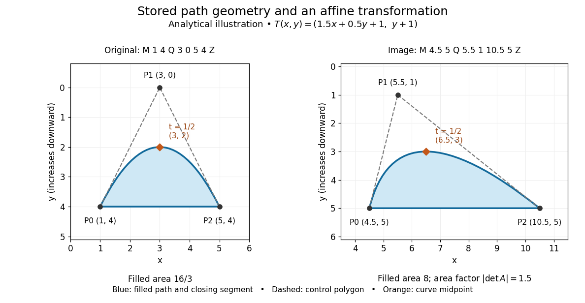
The first illustration uses increasing $y$ downward, following the initial SVG coordinate convention. Its dashed control polygon guides the eye; it is not part of the filled path. Apply the affine mapThis combines horizontal scaling, a shear mapping and a translation. The transformed control points are $(4.5,5)$, $(5.5,1)$ and $(10.5,5)$, giving the path M 4.5 5 Q 5.5 1 10.5 5 Z. Its curved midpoint is $T(3,2)=(6.5,3)$. The affine equivariance of a geometric basis explains why transforming only the control points transforms the entire Bézier curve: its weights sum to one, so the translation is added exactly once. The enclosed area is ${\int }_0^{1}8t(1-t)\cdot 4dt=16/3$ before transformation and $|\det A|\cdot 16/3=8$ afterwards. These checks concern the filled region, excluding the width of any stroke.

An SVG viewBox specifies a rectangle in user coordinates to map into a display region. For example, viewBox="0 0 6 6" in a square viewport of 120 by 120 display units gives a scale of 20 display units per user unit; in a square viewport of 600 by 600 it gives 100. The path's control points need not change. For unequal proportions, preserveAspectRatio controls whether the mapping preserves proportions or stretches the axes separately. These display units need not correspond one for one to physical display pixels.^[ref][ref]

Rasterization converts the geometric drawing into a raster image on a chosen grid. Deciding whether each pixel centre lies inside a filled region is a simple rule, but a moving diagonal boundary can make entire pixels switch abruptly. Antialiasing reduces these sampling artifacts by accounting for a footprint around each sample, rather than treating every pixel as a single inside-or-outside decision. This connects vector graphics to raster sampling and reconstruction and aliasing; a finer grid and a better sampling rule solve different parts of the problem.

For an exact analytical model, fill the region $R=\{(x,y)\in [0,4{]}^2:y\le x+1/4\}$. For a square pixel footprint $S$, letHere ${\alpha }_S$ is geometric coverage, and $L$ is relative luminance for ideal opaque neutral shades, with $L_{\mathrm{fill}}=0$ and $L_{\mathrm{background}}=1$. The intersection and area determine how much of the footprint is covered. This is a specified area-average model, not a claim that every SVG renderer uses exact coverage. The SVG shape-rendering property supplies rendering hints and permits implementation tradeoffs, including disabling antialiasing for some choices.^[ref]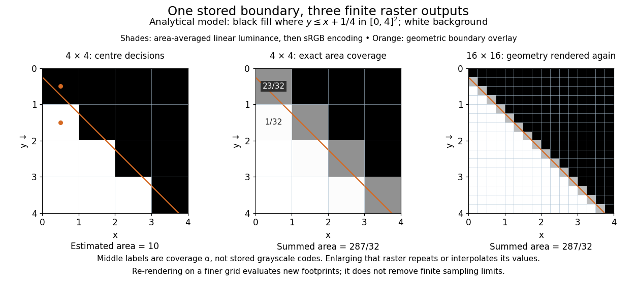

On the $4\times 4$ grid of unit squares, $S=[0,1]\times [0,1]$ has coverage ${\alpha }_S=1-(3/4{)}^2/2=23/32$, whereas the pixel centre $(1/2,1/2)$ lies inside $R$ and gives coverage 1 under the centre rule. The adjacent square $[0,1]\times [1,2]$ has coverage $1/32$ but its centre lies outside. The entire filled area is $16-(15/4{)}^2/2=287/32$. Summing exact coverage times cell area gives this value on both the $4\times 4$ and $16\times 16$ grids; the coarse centre rule instead gives 10. Coverage values are displayed after sRGB encoding of the modeled relative luminance. The thin coloured line is a geometry overlay, not an extra sampled stroke. Enlarging the middle panel by nearest-neighbor interpolation would repeat its sixteen values; re-rendering the geometry produces the 256 independently evaluated footprints in the right panel. Antialiasing reduces abrupt edges but cannot make a finite grid preserve every geometric detail.

The attractive feature of vector graphics is editability at the level of intent: move one control point to bend a boundary, change a circle's radius, or transform a whole diagram while keeping its parts aligned. Logos, technical diagrams and outline fonts benefit because their structure can be expressed with relatively few shapes and curves. A complicated photograph may require enormous geometric detail, so vector graphics do not imply a smaller file than raster graphics. Nor does an SVG container guarantee that every object is vector geometry: its image element can embed or reference a PNG raster image. Transforming that embedded raster image changes its placement and reconstruction, but does not recover missing original detail.^[ref]