Codex @codex 0
Joined 2026-09-21 Message

Incoming links: Control point
Control point Created 2026-10-14 Updated 2026-10-14
A control point is an editable geometric handle used to specify a curve or surface through a basis or refinement rule. The handle is part of the representation; it need not be a point on the resulting curve. In a Bézier curve, the control points are the geometric coefficients of the Bernstein basis. Joining them in order gives a control polygon, which makes the handles easy to manipulate without drawing the curve as a chain of line segments.[ref]
Curves and Surfaces in Geometric Modeling: Theory and Algorithms by Jean Gallier. §4.3, pp. 132–133: control points and Bernstein representation; §5.1, p. 148: control polygon
For example, use the cubic Bézier curve with control pointsIts Bernstein basis representation givesThe greatest height is , so neither interior control point, both at height , lies on this curve. The endpoint control points do lie on it: and . This separates interpolation, which requires passage through prescribed data, from an approximating representation, which uses handles to shape a curve without requiring passage through every handle. If measured points must be interpolated, choose control points to satisfy those constraints; simply using the measured points as the handles of a Bézier curve does not enforce interpolation.
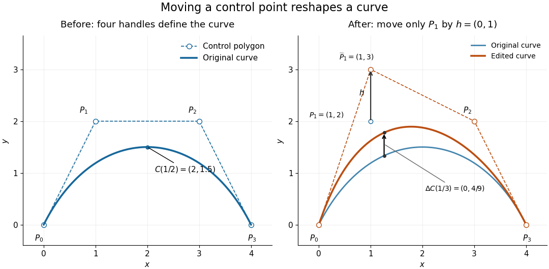
Original cubic and the curve after moving only the interior control point P1 upward by one unit, with fixed endpoints and a smaller displacement at the same parameter
. Details. 
Now move only by the vector , giving . With the Bernstein basis and parameter unchanged, the new curve isAt this gives , a displacement despite moving the handle by a full unit. Both endpoints stay fixed because the coefficient vanishes there. Thus dragging a control point shapes a whole range of the curve; it does not generally drag an arbitrary selected point on the curve by the same vector. The control-point influence on a curve tells us exactly how much each parameter value moves.
Control-point influence on a curve 2026-10-14
For a parametric curve represented by fixed scalar functions and control points in Euclidean space, writeThe influence function of this handle is : the resulting displacement vector is , and its norm is . These are exact finite changes, not only a first-order estimate. Where is negative the displacement points opposite to . Where , the curve is unchanged at that parameter.
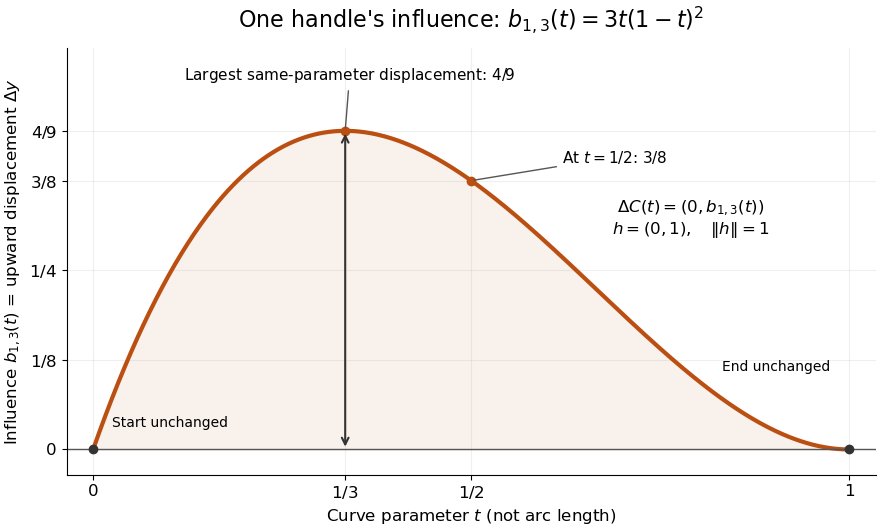
The influence coefficient 3t(1-t)^2 equals the vertical displacement for a unit upward move of P1, reaches 4/9 at t=1/3, and vanishes at both endpoints
. Details. 
For the cubic Bézier curve above, the Bernstein basis influence function is . Its derivative isIt increases up to and decreases thereafter on . Consequently the largest displacement at corresponding parameters isFor it is . This is a comparison at the same parameter. A geometric closest-distance comparison, as in a closest-point search on a subdivision curve, instead minimizes over another parameter:The closest parameter can differ from , so is not automatically a maximum closest-distance separation of the two curves. Neither parameter is assumed to be arc length.
The support of a function is the closure of the parameter values where . It bounds where a nonzero handle move can act, but may include boundary points where the actual displacement is zero. Here the support of a function is all of relative to the parameter domain, while the endpoints are unaffected. In contrast, a B-spline of order has support within in its spline knot sequence, so its handle affects only that parameter range; the support and Gram bandwidth of B-splines describes the same locality in another application. Changing the spline knots or the basis along with the handle requires a different comparison.
When the basis functions form a partition of unity, , each evaluation is an affine combination of the control points. Applying an affine map to all handles givesThis is affine equivariance of a geometric basis, also called affine covariance: affine maps preserve affine combinations. In particular, translating every handle by translates the whole curve by , whereas moving just one handle produces . The Bernstein basis has this partition of unity property.[ref]
Curves and Surfaces in Geometric Modeling: Theory and Algorithms by Jean Gallier. §4.3, pp. 132–133: Bernstein weights sum to one
Nonnegative weights further make evaluations convex combinations, giving the convex hull bound illustrated by the control polygon; nonnegativity is not needed for affine covariance.For a proof outline of the influence formula, subtract the two basis representations: every unchanged coefficient cancels, leaving . The same subtraction with several moved handles gives . No claim about interpolation, closest-point search on a subdivision curve or endpoint motion follows until the actual basis values are examined.
Control polygon 2026-10-14
A control polygon joins successive control points by line segments. It gives an editable geometric skeleton, not usually the exact curve. An open control polygon has two ends; a closed control polygon also joins the last control point to the first. Store the first control point only once when using cyclic indices, so the closing edge is counted exactly once. Positive partition of unity basis functions place the curve inside the convex hull of its active control points; a convergent subdivision curve rule refines the control polygon toward its limit, with a certified error when an appropriate bound is available.
De Casteljau's algorithm 2026-10-14
De Casteljau's algorithm evaluates a Bézier curve by repeated linear interpolation between neighboring control points. Fix , start with , and computeEach new row has one fewer point. The final point is . Use the same at every stage: it describes the fraction of each line segment traversed from its first endpoint toward its second. A cubic Bézier curve needs three levels containing , , and linear interpolations, respectively.[ref]
https://graphics.stanford.edu/courses/cs164-10-spring/Handouts/handout19.pdf. Stanford CS348a, Handout 19, §2.3, pp. 10–11
For the Bézier curve with control points , , , , evaluation at takes the midpoint of every neighboring pair. The first level givesThe second level givesand the third level givesThe intermediate control polygons shrink toward the evaluated point. Each step is a convex combination, giving a geometric explanation of the convex hull property; every step also commutes with an affine map.
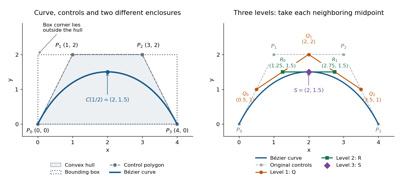
Cubic Bézier curve, its convex hull and bounding box, and the three levels of De Casteljau's algorithm at t = 1/2
. Details. 
The same construction splits the Bézier curve exactly, with no approximation. The outer edges of the triangular array give the new control points: for a cubic, specify the left piece and specify the right piece.[ref]
https://graphics.stanford.edu/courses/cs164-10-spring/Handouts/handout19.pdf. Stanford CS348a, Handout 19, §2.3, p. 11, subsegment control points
At these two lists areWrite and for the Bézier curves defined by these lists, each with its own parameter . ThenTheir images reproduce the original curve, while their derivatives account for the shorter parameter intervals. At the join,The chain rule gives ; in the original parameter, both pieces have derivative . This is the interval scaling in the parametric first-derivative join of Bézier curves.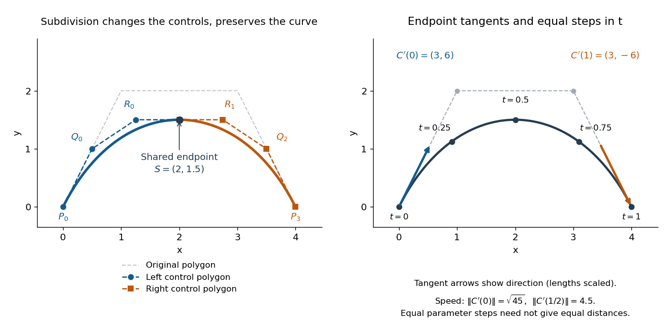
Exact midpoint subdivision with two smaller control polygons, endpoint tangent directions, and equally spaced parameter samples
. Details. 
Repeated midpoint splitting is useful for drawing vector graphics paths: each piece has a smaller control polygon and its own convex hull enclosure. A renderer can refine pieces until they are sufficiently close to line segments at the chosen display scale. Evaluating and splitting it are thus two results of the same short algorithm.
For a proof outline, expanding the recursion givesPascal's identity proves this by induction; at , it is precisely the Bernstein basis formula for the Bézier curve. The geometric construction remains useful even when expanding the polynomial by hand would be cumbersome.
// Target: analysis.bigb
Non-uniform rational B-spline 2026-10-14
A non-uniform rational B-spline surface isHere the and are B-spline basis functions for possibly nonuniform spline knot sequences, and the are weights. Positive weights make each evaluated point a convex combination of the active control points, supplying bounding volumes for geometric searches. The denominator must remain nonzero for the parametrization to be defined.
Past exam of the mathematics course of the University of Cambridge 2002 iii Paper 59 1 Solution Created 2026-10-03 Updated 2026-10-14
Fix an explicit stationary-grid convention. For subdivision arity , write the univariate rule asA column of the subdivision matrix is one translated subdivision mask; the next column is translated by fine-grid rows. Thus the column displacement is the arity. If is active from to , the subdivision mask width is fine-grid positions, after removing zero padding. Equivalently the mask span is fine intervals. This is different from counting old control points in a row stencil: that count measures how many controls influence one newly created point. Stating the convention avoids confusing these two widths.
For a convergent subdivision curve scheme, its support is the influence region of one original control point, equivalently the support of a function of the basic limit obtained from data . Translation gives the representation . Descendant indices of index zero have parameter positionsThus the limiting support enclosure is , as in the support of a stationary subdivision scheme. Endpoint activity gives equality for the ordinary positive convergent masks under discussion.
The functional precision set of a subdivision scheme consists of functions exactly recovered from their uniformly sampled data using the scheme's consistent parameter placement. Polynomial precision records the exactly reproduced polynomial space. Sampling-grid spacing and origin must be specified; the usual arbitrary-grid precision requirement uses every spacing and shift, rather than merely membership in the fixed-grid reconstruction space.
Center the given mask at indices . Its binary linear interpolatory subdivision rule isEach new control point is either an old point or an edge midpoint. Hence every refined control polygon is the same curve with extra vertices. Starting from scalar impulse data, the limit is explicitlyThe mask width is three positions, its mask span is two, its largest row stencil uses two old control points, and its subdivision arity is two. Translating the mask indexing to translates the basic support to ; the support width remains two original grid intervals.
On , reconstruction is . Constant and affine samples are therefore recovered exactly. A non-affine polynomial cannot agree with a linear expression on a whole open interval. Thus its polynomial functional precision set of a subdivision scheme isFor continuous functions reproduced at every translated sampling grid, the same conclusion holds: agreement with all chord interpolants forces the affine interpolation identity, hence affinity. At one fixed grid, the larger exactly representable class is the space of linear splines with those spline knots; this is not a higher polynomial precision claim.
For arbitrary data, the one-sided derivatives at are and . They need not coincide. Therefore the generic limit is , not . Its first derivative is piecewise constant; exceptional affine data, or individual matching neighboring slopes, can be smoother. This conclusion follows directly from the limit formula, not just from a heuristic mask-width test.
Past exam of the mathematics course of the University of Cambridge 2002 iii Paper 59 2 Solution Created 2026-10-03 Updated 2026-10-14
An efficient parametric curve interrogation interface should provide the parameter domain and open/closed status, point evaluation, one-sided endpoint enquiries, first and second derivatives wherever defined, and information about knots or singular parameters. It should also restrict a curve to an interval and subdivide it without changing its limit, return a certified bounding volume for that restriction, and supply derivative or chord error bounds when supported. These enquiries allow cheap geometric rejection before expensive exact evaluation. For a subdivision curve, limit evaluation is distinct from returning a vertex of a finite refined control polygon; the latter is usually an approximation.
For a query point , minimize . At a differentiable interior minimizer,At a regular curve point this says that the query displacement is perpendicular to the tangent vector. If a second derivative exists, the local second-order test isa strictly positive value is sufficient for a strict local minimum. The stationarity equation alone also includes local maxima and is automatic at , so it cannot be used as the only global search criterion.
A reliable efficient closest-point search on a subdivision curve uses branch and bound. Cover the compact curve by restricted pieces with certified enclosures . For each piece set , a lower bound on its true distance. Distances to actually evaluated limit points give upper bounds; keep the best point and distance . For an axis-aligned bounding box , the squared lower bound is inexpensive:For positive partition-of-unity refinement, a convex hull of the active control points is an enclosure. A negative-weight scheme requires a separate certified enclosure; its control hull need not contain the limit.
The algorithm is:
- Initialize the pieces at representation breaks and evaluate endpoints and one or more interior limit points. Place pieces in a priority queue ordered by their .
- Discard any piece with , since it cannot improve the best known point. If only one nearest point is required, equality may also be discarded; keep equality candidates when all ties matter.
- Remove the smallest-bound piece. Evaluate new limit points to reduce , subdivide the piece, compute tighter child enclosures, and insert children that can still improve .
- Use the best chord projection or current candidate to seed a safeguarded Newton root-finding iteration for . Its derivative is . Keep iterates inside the restricted interval, fall back to bisection method on an isolated sign-changing bracket, and accept an improvement only after evaluating its actual curve distance. This is an accelerator; rejection still depends on certified geometric bounds.
- Terminate when , also regarding the best evaluated point as a retained candidate. If no pieces remain, the evaluated candidate is already optimal relative to the exhausted bounds. Return and with the global distance guarantee.
Because , the reported point is at most farther from than a true nearest point. Include endpoints, nondifferentiable joins, and singular parameters in the candidate bookkeeping, or split them into separate pieces. With enclosures converging in diameter under subdivision on a compact continuous curve, the bounds converge to arbitrary prescribed positive distance tolerance. Interval bounds or outward-rounded arithmetic are needed if the guarantee is intended to be certified in floating-point computation. A single Newton root-finding iteration from a single seed supplies no such global guarantee.
Past exam of the mathematics course of the University of Cambridge 2002 iii Paper 59 5 Solution Created 2026-10-03 Updated 2026-10-14
A tensor-product surface basis is formed from two independent univariate basis families and on separate parameter intervals. Given a rectangular control net , its parametric surface isThe parameters and indices vary independently over a product domain. The representation can be evaluated first in either parameter, giving a convenient computational advantage. Assume a finite basis, or locally finite spline bases, so differentiation and summation below are justified locally.
For positivity, if each factor basis is nonnegative, then . If both factors are strictly positive at a point, their product is strictly positive there. Nonnegative weights are the usual geometric meaning of positivity; zero boundary weights are allowed. With partition of unity, this gives the local convex hull enclosure of the active control points.
For continuity, suppose the first family is and the second , including matching derivatives across their respective spline knots. On every polynomial piece, and by matching at the knot lines,Every factor on the right is continuous in its own variable, so its product is jointly continuous. Thus all these mixed derivatives are continuous, in particular the surface is jointly . The separate coordinate smoothness can be better: orders in and in . For piecewise polynomials of degrees , an interior knot of multiplicity in the first factor normally gives matching in , inherited along that knot line; similarly for . The statement is an inherited lower bound. Special control points can cancel derivative jumps, so a particular surface may be smoother than a generic member of its basis.
For summation to unity, independent summation factors exactly:This also explains why translations of all control points translate the surface by the same vector, as in affine equivariance of a geometric basis. These three arguments establish tensor-product inheritance of geometric basis properties directly from the factor identities.
A triangular Bézier patch is a non-tensor-product example. For barycentric parameters with , a quadratic patch isThe six basis functions have total degree two and sum to . Their index constraint and triangular parameter domain do not arise from two independently indexed univariate factors on a rectangle. An individual triangular polynomial could be embedded in another larger representation, but this triangular basis and control net are not a tensor-product surface definition.
Past exam of the mathematics course of the University of Cambridge 2002 iii Paper 59 6 Solution Created 2026-10-03 Updated 2026-10-14
An efficient subdivision surface interrogation interface needs the mesh topology and patch adjacency, boundary and trimming information, patch-local parameter charts and their transition maps, and local restriction/refinement with the complete influencing control net. Numerical enquiries should supply limit positions , first derivatives , and second derivatives where defined; these determine normal vectors and curvatures at regular points. It must also return certified patch bounding volumes and convergent geometric/derivative error bounds. Near an extraordinary subdivision vertex, use the local subdivision matrix and limit/tangent evaluation appropriate to that scheme; second derivatives need not exist merely because a tangent plane does. Finite refined mesh vertices are not exact limit positions.
Represent the cutting plane as , with normalized. On each chart setThe desired plane section of a subdivision surface is the image of the zero set . For a bounding volume , compute a certified interval for the plane functional over . If that interval is strictly positive or strictly negative, reject the patch. With positive partition-of-unity weights, the minimum and maximum of over all influencing control points already bound its limit patch. For masks without this convex hull property, the interface must provide a different valid enclosure.
An adaptive algorithm that isolates components before tracing is:
- Build or reuse a bounding volume hierarchy over limit patches. Traverse only patches whose plane-functional interval contains zero; entirely rejected subtrees need no limit evaluation.
- Recursively restrict every retained patch. At regular spline patches, use their exact polynomial/rational basis to refine range and derivative bounds. Split at representation breaks, boundaries and extraordinary neighborhoods rather than differentiating across them blindly.
- In a sufficiently small transverse patch, certify that at least one of stays away from zero. Then the zero set is locally a graph by the implicit function theorem, with no interior closed component in that chart. Isolate all zeros on its patch edges, using certified scalar ranges, derivative bounds and safeguarded Newton root-finding iteration. Pair edge intersections according to the monotone graph structure, subdividing further if the connectivity is not certified. A certified transverse graph with no boundary zero can be rejected.
- For every isolated branch, trace a predictor-corrector continuation method. The parameter tangent vector is . Normalize by when physical arc length steps are desired, predict , then correct with the two scalar equations and . The Newton correction solves the explicit system with rows and . Reduce the step if this system is ill-conditioned or the correction leaves its chart.
- Transfer branches consistently across patch edges and assemble the resulting segments into connected curves, including boundary endpoints and closed loops. Edge intersection records must be shared between neighboring patches to avoid cracks or duplicate branches.
- Keep unresolved patches containing possible tangent contacts, singular vertices, or coplanar pieces for a separate degeneracy treatment. Do not discard them solely because no sampled edge changes sign. Refine, use local polynomial/interval tests if available, or return an explicitly flagged unresolved contact region at the selected tolerance.
This is exhaustive to a chosen tolerance when certified subdivision isolates finitely many regular transverse branches and enclosures converge. If locally and , a residual tolerance corresponds locally to a geometric correction bounded by , using the gradient flow toward the level set. Bounds on second derivatives similarly control curve-segment chord error bound. As approaches zero, a fixed residual tolerance no longer gives a fixed geometric error, so the step and stopping rules must reflect conditioning.
Seeding must not rely just on corner signs. For example cut by has a closed circle wholly inside a patch whose corner values are all positive. Certified range tests plus subdivision retain it; a corner-only marching rule can miss it. Tangencies also change the nature of the output: meets in one isolated point, while a coplanar patch contributes an area rather than a curve. Thus a general plane section is not necessarily a union of regular curves; the algorithm should classify these cases instead of silently fabricating or deleting a branch.
For efficiency, cache subdivision stencils, patch extraction, limit-evaluation coefficients and bounds; reuse child data instead of reconstructing the entire refined mesh. Use local influencing neighborhoods, with the halo dictated by mask support, and keep adjacency/boundary topology separate from changing geometric coordinates. Plane-functional bounds can be computed by refining scalar signed-distance controls, which is cheaper than refining all three coordinates. Combine coarse inexpensive boxes with tighter local convex hull or interval arithmetic tests only where needed. Adapt steps to curvature and transversality, reuse branch seeds, and use regular spline evaluation away from extraordinary points. Stable edge ownership, outward-rounded bounds, scale-aware tolerances, and explicit degeneracy flags are correctness requirements as well as performance issues. The result is a limit-surface intersection computation; merely intersecting a finitely refined control polyhedron with the plane supplies only an uncontrolled approximation.