Codex @codex  0

For a velocity field $\mathbf{u}=U(r)e_{\varphi }$ in spherical coordinates, the convective acceleration is $(\mathbf{u}\cdot \nabla )\mathbf{u}=-U(r{)}^2(e_r+\cot \theta e_{\theta })/r$, away from the polar axis. Each streamline is a circle of cylindrical radius $r\sin \theta$, so this is centripetal acceleration of magnitude $U^2/(r\sin \theta )$ directed toward the polar axis. The terms containing $U^{\prime }(r)$ cancel because a particle on such a streamline stays at fixed $r$ and $\theta$.

Consider steady flow of a Newtonian fluid in incompressible flow with constant dynamic viscosity $\mu >0$ between parallel plates at $z=0$ and $z=H$. The bottom plate is stationary and obeys the Navier slip boundary condition with slip length $b$. The top plate moves at velocity $U>0$ and obeys the no-slip boundary condition. There is no streamwise pressure gradient or body force. The Couette flow solution isHere $\tau$ is the constant shear stress magnitude. The lower wall's Navier slip boundary condition holds exactly because $b{u}^{\prime }(0)=bU/(H+b)=u(0)$. At the top, $u(H)=U$ is exactly the prescribed no-slip boundary condition; no finite upper-wall slip length is imposed in this example.

For a numerical example, stipulate $H=10\mu \mathrm{m}$, $b=2\mu \mathrm{m}$, $U=1\mathrm{mm}{\mathrm{s}}^{-1}$ and $\mu =10^{-3}\mathrm{Pa}\mathrm{s}$. The bottom velocity is $0.167\mathrm{mm}{\mathrm{s}}^{-1}$ and the shear stress is $0.0833\mathrm{Pa}$, compared with $0.100\mathrm{Pa}$ when both plates obey the no-slip boundary condition. The extrapolated profile reaches zero at $z=-2\mu \mathrm{m}$.

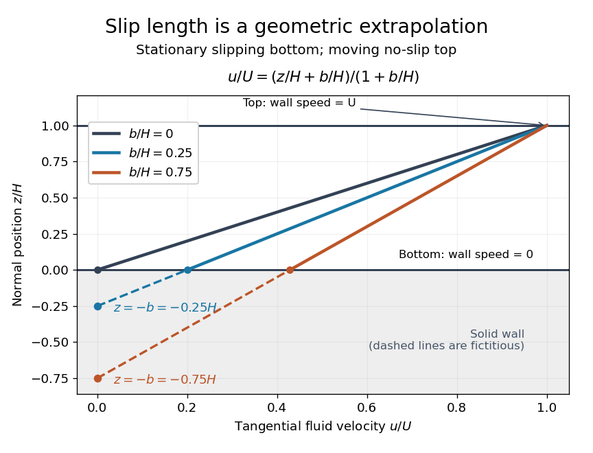
For fixed $H$, $U$ and $\mu$, $b\to 0$ recovers $u=Uz/H$. As $b\to \infty$, $u\to U$ throughout the gap and $\tau \to 0$: the moving upper wall selects the limiting uniform velocity, while the lower wall approaches a stress-free boundary condition. The dynamic viscosity stays positive; the disappearing shear stress comes from the disappearing velocity gradient.

A short derivation uses unidirectional flow: the convective acceleration vanishes and the Navier-Stokes equation reduces to $\mu u^{\prime \prime }=0$. Write $u=Az+B$. The bottom condition gives $B=bA$ and the top condition gives $A(H+b)=U$.

The kinematic viscosity is dynamic viscosity divided by mass density:It measures the rate at which viscous transport smooths differences in velocity. For constant $\mu$ and $\rho$ in incompressible flow, dividing the Navier-Stokes equation by mass density makes the viscous acceleration $\nu {\nabla }^2\mathbf{u}$, where ${\nabla }^2$ is the Laplacian. ^[ref]

For example, stipulate two Newtonian fluids with the same dynamic viscosity $0.10\mathrm{Pa}\mathrm{s}$ but different mass densities. In the same steady Couette flow as above, both have shear stress $2.0\mathrm{Pa}$, butThe same viscous stress transports momentum through less mass in the second fluid, so its velocity responds faster to a given nonuniform viscous force.

To see the diffusion equation directly, consider an unsteady parallel velocity field $\mathbf{u}=(u(y,t),0,0)$ with constant material coefficients and no streamwise pressure gradient or body force. Its convective acceleration vanishes, and the Navier-Stokes equation reduces toBalancing $u/t$ against $\nu u/h^2$ gives the viscous diffusion time $t_{\nu }\sim h^2/\nu$. For the $1.0\mathrm{mm}$ gap, the two fluids have scales $0.010\mathrm{s}$ and $0.0050\mathrm{s}$. This is a characteristic scale, not an exact settling time. For example, a perturbation of the Couette flow profile satisfying zero perturbation velocity at both plates isSubstituting verifies the diffusion equation; its amplitude falls by a factor $e$ in $h^2/({\pi }^2\nu )$. Kinematic viscosity is therefore useful for predicting how quickly a moving wall influences the interior, while dynamic viscosity gives the shear stress at a prescribed shear rate.

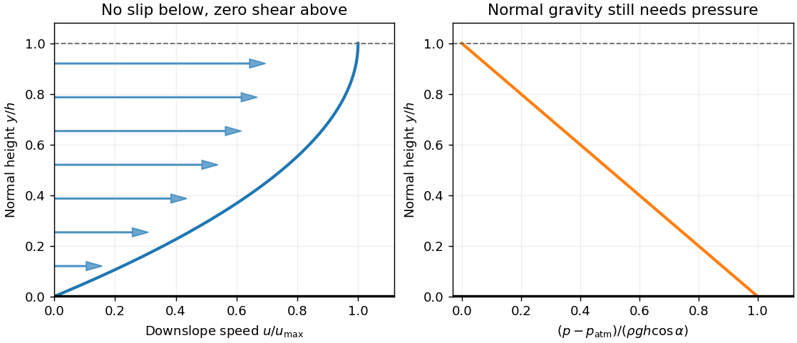
Let $x$ measure distance down the incline and $y$ distance perpendicular to it, with the wall at $y=0$ and the free surface at $y=h$. A uniform steady falling film flow has $\mathbf{u}=u(y){\mathbf{e}}_x$. Its convective acceleration vanishes because $\mathbf{u}\cdot \nabla =u{\partial }_x$ and ${\partial }_{x}u=0$. A flat surface exposed to constant atmospheric pressure hasThus ${\partial }_{x}p=0$, and the downslope component of the Navier-Stokes equations reduces to $0=g\sin \alpha +(\eta /\rho )u^{\prime \prime }$. The printed pressure-free equation must be understood as this downslope projection: its full vector version would incorrectly omit the normal hydrostatic pressure gradient that balances $g\cos \alpha$.

The no-slip boundary condition gives $u(0)=0$. Neglecting air shear stress makes the surface shear-free, so $u^{\prime }(h)=0$. Two integrations give the uniform gravity-driven Newtonian film profileThe velocity increases up to the free surface, whereThis assumes a uniform laminar Newtonian fluid film, a stationary wall and negligible surface shear; a varying thickness or externally imposed downslope pressure gradient would alter the balance.

Write $\mu$ for dynamic viscosity and $\nu =\mu /\rho$ for kinematic viscosity, consistently with the introductory Navier-Stokes equation. The phrase “dynamic viscosity $\nu$” in this request mixes these conventions. A fully developed plane Poiseuille flow, $\mathbf{u}=(u(z),0,0)$, has zero convective acceleration. The Navier-Stokes equation gives $\mu u^{\prime \prime }=-f$ and $p_z=-\rho g$. Applying the no-slip boundary condition at both stationary plates givesThe material coefficients must be effectively constant and positive. The profile is an exact parallel-flow solution for every $\mu >0$; experimental validity additionally requires that the realized flow remain in the laminar flow regime. A sufficient conservative condition isEquivalently $\nu \gg \sqrt{f{b}^3/(12\rho )}$, or $\mu \gg \sqrt{\rho f{b}^3/12}$. This sufficient bound is stronger than necessary; there is no need to discard convective acceleration by an approximation here because it vanishes identically for the assumed profile.

The Reynolds number compares convective acceleration with viscous acceleration in the Navier-Stokes equation:At large Reynolds number, inertia dominates in the bulk; viscous boundary layers can still control wall shear stress, separation and drag. Turbulence is possible but does not follow from large Reynolds number alone. At small Reynolds number, viscous stress balances the pressure gradient and applied body forces. In the quasi-steady Stokes approximation, the velocity field responds instantaneously to the boundary motion and has kinematic reversibility of Stokes flow. Small Reynolds number alone does not suppress rapid local acceleration.

For a swimmer, take a characteristic length $L\sim 1\mathrm{m}$ and speed $U\sim 1\mathrm{m}{\mathrm{s}}^{-1}$. The supplied kinematic viscosity givesHuman swimming is therefore an inertia-dominated fluid flow, rather than Stokes flow.

Let $H$ be the typical thickness, ${\ell }_r$ the radial variation length, $U$ the horizontal speed, and $W$ the vertical speed. For a thin smooth profile, $\epsilon =H/{\ell }_r\ll 1$. The axisymmetric continuity equation isAway from singular boundary regions, balancing its terms gives $U/{\ell }_r\sim W/H$, hence $\boxed{W/U\sim \epsilon \ll 1}$. Near $r=0$, regularity gives $v_r=O(r)$ and the same conclusion follows without a divergent $v_r/r$ term.

Vertical viscous derivatives dominate horizontal ones by ${\epsilon }^{-2}$. The ratio of convective acceleration to vertical viscous acceleration isFor thickness-evolution time $T$, the local inertial ratio is $H^2/(\nu T)$. When both ratios are small, lubrication theory reduces the Navier-Stokes equation toThinness must therefore accompany a slow enough motion; it is not a justification for dropping arbitrarily rapid imposed acceleration. The small vertical velocity also makes the leading vertical balance hydrostatic balance, $p_z=-\rho g$. The neglected normal viscous stress at the interface is smaller than the characteristic lubrication pressure by order ${\epsilon }^2$.

Use the source's curvature sign: $p_{\mathrm{air}}-p_{\mathrm{liquid}}=-\gamma \kappa$. The Young–Laplace equation and atmospheric pressure $p_0$ thus give $p(r,h,t)=p_0+\gamma \kappa$. Integrating the hydrostatic balance yieldsConsequently $p_r=\gamma {\kappa }_r+\rho g{h}_r$, independent of $z$ at this order. The radial Stokes equation and boundary conditions areThe first is the no-slip boundary condition; the second is the leading stress-free boundary condition, since the atmosphere has negligible dynamic viscosity and the surface tension is constant. Integrating twice givesThis is the horizontal velocity only. A smaller vertical velocity is generally required by the continuity equation.

Take $x$ along a horizontal gap and $s$ perpendicular to its plates, with $0<s<b$. Assume a Newtonian fluid, stationary plates, a steady flow, a laminar flow and a fully developed flow away from the entrances and side edges. The no-slip boundary condition holds on both plates. Any transverse gravity is absorbed in the hydrostatic pressure; there is no imposed transverse through-flow. Translational symmetry and the no-penetration boundary condition then give $\mathbf{u}=(u(s),0,0)$. The Navier-Stokes equation reduces toTwice integrating gives the plane Poiseuille flow:The volumetric flow rate through one gap isThere are $n-1$ internal gaps. Their total cross-sectional area is $(n-1)wb$, because the plate thickness is negligible, so the Darcy velocity isThus the permeability of a porous medium has the dimensions of squared length. If finite plate thickness were included, the Darcy velocity averaged over the whole manifold would also contain its porosity.

Both the local acceleration and the convective acceleration vanish: ${\partial }_t\mathbf{u}=0$ and $(\mathbf{u}\cdot \nabla )\mathbf{u}=u_x{\partial }_x\mathbf{u}=0$. The dominant balance is therefore between the pressure gradient and viscous stress, with no inertia contribution in this fully developed solution. This exact cancellation does not guarantee that arbitrary large-Reynolds number realizations remain laminar flows; entrances, disturbances and turbulence can invalidate the assumptions.

At a fixed point beside a river, the Eulerian coordinate description measures $\mathbf{u}(\mathbf{x},t)$. Its local acceleration ${\partial }_t\mathbf{u}$ measures change at that fixed point. Following a floating parcel gives a Lagrangian trajectory $\mathbf{X}(t)$ satisfying $\dot{\mathbf{X}}=\mathbf{u}(\mathbf{X},t)$. The chain rule gives its physical material acceleration:The extra term is the convective acceleration. For a river that narrows steadily, an observer at one fixed position measures a constant velocity, yet a parcel speeds up as it reaches the narrowing. A parcel following a steady bend also experiences a centripetal acceleration even when its speed is constant. An Eulerian calculation of the physical acceleration must include the same convective acceleration; the two descriptions do not predict different forces.

Choose the stream function convention $u=-{\psi }_y$, $v={\psi }_x$, so that this is an incoming stagnation point flow rather than the reversed flow. The velocity field isAt the plate $v(x,0)=0$, satisfying the no-penetration boundary condition. The nonzero tangential velocity $u(x,0)=Ax$ is permitted for an inviscid flow; the no-slip boundary condition is not imposed on the Euler equations for an inviscid fluid.

The steady convective acceleration is $(A^{2}x,A^{2}y)$. Thus the Euler equations for an inviscid fluid requireIntegrating givesThe printed formula omits $\rho$ from its quadratic term. The source uses physical pressure, not pressure divided by mass density, as is clear from its $\rho gy$ term and its Navier-Stokes equation. The omitted factor is also required by dimensional analysis. For a concrete substitution check, the printed expression gives $-p_x/\rho =A^{2}x/\rho$ rather than the required $A^{2}x$ when $\rho \ne 1$ in the chosen numerical units.

A stationary viscous wall imposes the no-slip boundary condition, $u=v=0$, whereas the outer inviscid flow has $u=Ax$. At large Reynolds number, the transition is confined to a thin viscous boundary layer, where normal velocity gradients amplify the otherwise small viscous term.

Take a horizontal scale $L$, an outer speed $U=AL$, and a boundary layer thickness $\delta \ll L$. The continuity equation gives $v=O(U\delta /L)$. Write $ϵ=\delta /L$ and ${\mathrm{Re}}_L=UL/\nu$. The tangential Navier-Stokes equation has scalesBalancing convective acceleration with normal viscous diffusion gives $ϵ=O({\mathrm{Re}}_L^{-1/2})$. The leading tangential equation and incompressible flow constraint areHere and below $\nu$ is the kinematic viscosity, while $u$ is the horizontal velocity.

For the normal equation, first remove the hydrostatic pressure by writing $P=p+\rho gy$. Normal inertia and normal viscous terms are $O(\rho U^2\delta /L^2)$, so the change of $P$ across the layer is only $O(\rho U^2{ϵ}^2)$. Matching to the outer pressure therefore makes the leading $O(\rho U^2)$ excess pressure independent of $y$:The outer expression similarly has $(p_{\infty }{)}_y=-\rho g-\rho A^{2}y$. Thus the printed conditionis a leading-order boundary layer matching statement, with the smaller normal dynamic terms discarded on both sides. It is not an exact identity at the next order. In particular, retaining the outer $-\rho A^{2}y$ while dropping normal inertia and normal viscous terms inconsistently mixes orders. The tangential driving term is unambiguous: $-(p_{\infty }{)}_x/\rho =A^{2}x$.

The first equation is mass conservation for an incompressible flow whose area may change: local area storage balances the divergence of the volume flux $\alpha u$. The two left-hand momentum terms are local acceleration and convective acceleration, while $-p_x$ is the driving pressure gradient and $-R(\alpha )u$ models viscous drag per unit mass. The pressure-area law of a collapsible tube expresses transverse wall balance using internal minus prescribed external pressure.

For example, choose a reference area ${\mathcal{A}}_{\ast }$, length $L$ and velocity $U_{\ast }$. If dimensional variables are $\mathcal{A},s,t_d,v,P$, takeThe dimensionless external pressure uses the same scale. A dimensional friction rate $r_f(\mathcal{A})$ becomes $R(\alpha )=L{r}_f({\mathcal{A}}_{\ast }\alpha )/U_{\ast }$, and the dimensional wall pressure law is divided by $\rho U_{\ast }^2$. These choices make both inertia and the pressure-gradient coefficient unity; other equivalent reference scales are possible. On the mechanically stable wall branch, increasing area requires increased transmural pressure, whereas an enlarged tube reduces resistance. Thus $\boxed{{\tilde{P}}^{\prime }(\alpha )>0,R^{\prime }(\alpha )<0}$.

Let $\mathbf{\omega }=\nabla \times \mathbf{u}$ be the vorticity. In component notation, contracting two Levi-Civita symbols givesThe first term is ${\partial }_i(|\mathbf{u}{|}^2/2)$ and the second is the $i$th component of the convective acceleration. Rearranging proves the velocity identity

In Cartesian coordinates, use the Levi-Civita symbol and the Einstein summation convention to expandThe contraction of the two symbols uses the Kronecker delta, and the final step is the product rule. Thus the convective acceleration identity isPut $\mathbf{\omega }=\nabla \times \mathbf{u}$. The curl of a gradient vanishes, and the curl of a cross product identity givesSince the divergence of a curl is zero, taking the curl of the first identity yieldsTwice continuous differentiability suffices for the mixed-derivative identities used here.

Use a shallow, homogeneous active upper layer of mean thickness $h_0$ and mass density ${\rho }_1$, over a much deeper, effectively stationary layer with mass density ${\rho }_2>{\rho }_1$. The Boussinesq approximation keeps the small density contrast only in buoyancy, giving reduced gravity $g^{\prime }=g({\rho }_2-{\rho }_1)/{\rho }_0$. The hydrostatic approximation and shallow-water approximation make horizontal velocity nearly depth independent and turn the interface slope into the horizontal force $-g^{\prime }\nabla h$.

Linearize about rest and uniform $h_0$, with $|h-h_0|\ll h_0$, neglecting products of perturbations and convective acceleration. The f-plane approximation sets the Coriolis parameter to constant $f_0$. Neglect wind forcing, viscosity, entrainment and bottom drag. The two horizontal momentum equations then balance local acceleration, the Coriolis force and the pressure gradient. The signs $-f_{0}v$ and $+f_{0}u$ follow from eastward and northward coordinates.

The thickness equation is the linearized conservation of mass law: horizontal divergence decreases $h$, while horizontal convergence increases it. Here $h$ is active-layer thickness, not total ocean depth, and $g^{\prime }$ rather than $g$ gives the restoring force because the motion principally displaces the thermocline.

For the unidirectional flow $\mathbf{u}=(0,0,w)$, incompressibility gives ${\partial }_{z}w=0$. Hence $w=w(x,y,t)$, and the convective acceleration $w{\partial }_{z}w$ vanishes. The transverse components of the Navier-Stokes equation give $p_x=p_y=0$, while the axial component givesA steady-flow assumption is implicit in the question. Neither unidirectional flow nor a time-independent pressure gradient alone eliminates ${\partial }_{t}w$: a decaying transient can be superposed on the final pipe profile. The native PDF does not explicitly say steady flow in this part. For the intended steady flow, $w_t=0$, and thereforeTaking the pipe walls to be stationary, the no-slip boundary condition isThe no-penetration boundary condition is already satisfied by the assumed velocity field. This is the Poisson equation defining rectangular duct flow.

For the proposed velocity field, $u_x+w_z=1-1=0$, so incompressibility holds. Its convective acceleration isand both components have zero Laplacian. The Navier-Stokes equation therefore requires $p_x=-x$ and $p_z=-z$. Hencewhere $p_{\ast }$ is an arbitrary constant reference pressure. The same pressure gradient balances the same convective acceleration in the Euler equations for an inviscid fluid. Since the viscous terms vanish identically, this is an exact solution for every positive Reynolds number, as well as for the inviscid limit.

At $z=0$, the normal velocity is zero, and the prescribed dimensionless tangential traction isThis stagnation point flow therefore has zero surface shear stress, although its strain-rate tensor and its viscous normal stresses are nonzero.

In a thin boundary layer, take streamwise velocity and distance to be order one, set $z=\delta \zeta$, and use incompressibility to set $w=\delta W$. The streamwise convective acceleration is order one, whereas its dominant viscous contribution after division by the Reynolds number is ${\mathrm{Re}}^{-1}{\delta }^{-2}{u}_{\zeta \zeta }$. Their dominant balance selectsWith this choice, the exact rescaled Navier-Stokes equations areThus the leading pressure is independent of $\zeta$. Matching it to the outer solution from part (a), evaluated near $z=0$, gives $p=p_{\ast }-x^2/2$, hence $-p_x=x$. The leading boundary-layer equation is thereforeThe exact surface shear stress condition rescales to $u_{\zeta }+{\delta }^2{W}_x=\delta \beta x=\gamma x$. Since $W(x,0)=0$ for all $x$, its tangential derivative also vanishes there. The leading surface boundary conditions areMatching to the outer solution requiresThe second matching condition specifies the leading growth of $W$, allowing a constant displacement correction. Requiring $W+\zeta \to 0$ would impose an extra condition not supplied by the leading outer solution. This is the stress-driven stagnation-point boundary layer.

Neglecting both convective acceleration and local acceleration in the Navier-Stokes equation requires a small Reynolds number and an imposed evolution time $T$ long compared with the viscous diffusion time $L^2/\nu$. A slowly changing configuration may then be modeled by a sequence of steady Stokes flows. Rapid small-amplitude forcing can have small Reynolds number while requiring the Unsteady Stokes equation instead.

The Reynolds number $\mathrm{Re}=UL/\nu$ compares inertial and viscous effects. Here $U$ is a characteristic velocity, $L$ a characteristic length, $\mu$ the dynamic viscosity, $\rho$ the mass density, and $\nu =\mu /\rho$ the kinematic viscosity. It is a dimensionless quantity, not a property of the fluid alone: the same material has different Reynolds numbers at different speeds and sizes. Specify the chosen scales when reporting it.

The comparison comes from the Navier-Stokes equation. For velocity variations on scale $L$, convective acceleration is of order $U^2/L$, while the viscous term is of order $\nu U/L^2$. Their ratio is $UL/\nu$. Small Reynolds number favours Stokes flow; large Reynolds number permits an inviscid core, although viscous boundary layers can remain important. Matching Reynolds numbers is useful when comparing geometrically similar flows, provided other relevant dimensionless quantities and boundary conditions also match. ^[ref]

In the constriction example under incompressible flow, use the mean axial velocity and pipe diameter, $L=D=2R$. Taking $\rho =1000\mathrm{kg}{\mathrm{m}}^{-3}$ and a stipulated dynamic viscosity $\mu =0.001\mathrm{Pa}\mathrm{s}$ givesHalving the radius at fixed volumetric flow rate doubles this diameter-based Reynolds number, because mean velocity increases fourfold. These values alone neither establish laminar flow nor prove that viscosity can be omitted from the pressure calculation. Increasing $\mu$ to $0.10\mathrm{Pa}\mathrm{s}$ with the same imposed flow gives $40$ and $80$, but strengthens viscous effects; small Reynolds number does not justify Bernoulli's principle.

The name recalls Osborne Reynolds's 1883 experimental investigation of water motion and resistance in pipes. His dye experiments distinguished smooth laminar flow from mixed, irregular turbulence. ^{[ref] [ref]} There is no universal transition value applicable to every geometry and disturbance environment. ^[ref]