Codex @codex  0

Use the zero initial displacement and velocity given in the PDF. The characteristic roots of the homogeneous equation are $-1\pm i\mu$. Its causal Green function of a damped oscillator iswhere $H$ is the Heaviside step function. The positive-time kernel has $G(0+)=0$ and $G^{\prime }(0+)=1$, so its derivative jump generates a unit impulse. The zero-data forced solution is consequently the causal convolutionDifferentiating once gives $x^{\prime }(0)=0$; differentiating twice supplies the endpoint term $g(t)$ and verifies the differential equation. No homogeneous transient is required with these initial data.

The filter is a real even triangular function. Its Fourier transform iswith $\tilde{f}(0)=1$. Since the transmitted pulse is the convolution $b=a\ast f$, the convolution theorem givesThe normalized filter preserves the time integral of the pulse, while its extra inverse-frequency factors suppress high-frequency content. It is a smoothing filter rather than an exact compact-bandwidth cutoff.

The pulse height is the constant $t_0$, not the time variable. In the undamped case the convolution therefore reduces toIntegration gives the continuous displacement and velocityThe post-pulse expression is equivalently $x(t)=(t_0/2)\sin t_0\sin (2t-t_0)$. Since $t_0>0$, it vanishes for every subsequent time precisely when $\sin t_0=0$. ThusThese are integer multiples of the oscillator's natural period $\pi$. At such switch-off times both $x(t_0)$ and $x^{\prime }(t_0)$ are zero. Vanishing displacement alone would not suffice: a nonzero switch-off velocity would restart an oscillation. This is rectangular-pulse cancellation of an undamped oscillator.

Suppose initially that $f,g$ are absolutely integrable, so Fubini's theorem justifies exchanging the integrations. The transform of their convolution isSet $s=z-t$, so $z=s+t$ and $dz=ds$. The exponential separates:Therefore the convolution theorem isNo extra $2\pi$ occurs in this direction with the specified normalization.

For the critically damped case, causality reduces the convolution toAlthough the forcing is not integrable on the full real line, this integral converges absolutely because the Green's function is integrable. Thus the calculation is valid directly; the corresponding Fourier transform can be interpreted as a tempered distribution.

Use the complex exponential and ${\int }_0^{\infty }s{e}^{-as}ds=a^{-2}$ for $\mathrm{Re}a>0$:Since $(1+i{)}^2=2i$, the convolution response isThis is the bounded steady response to the stated forcing acting for all time. Without an initial condition or the convolution selection, the general solution additionally contains $(C_1+C_{2}t)e^{-\kappa t}$. No switch-on at $t=0$ was specified, so zero initial displacement and velocity should not be imposed on this all-time forcing.

Assume initially that $f,g$ are integrable, so Fubini's theorem justifies interchanging the integrals. Transform the convolution and put $u=x-z$:This is the convolution theorem. No factor $2\pi$ appears in this direction because the forward transform in the question is unnormalized.

Let $r(z)$ be the indicator of $[-1,1]$. The finite integral is exactly the convolution $p=q\ast r$. Its additional transform factor isApplying the convolution theorem and part (d),Equivalently this is $2(\sin k/k)[\sin (k/2)/(k/2){]}^2$. The value at zero also follows from $\int p=(\int q)(\int r)=1\times 2$.

By the definition of convolution and Fourier inversion,The second line uses $\nu =\omega -\eta$. The factor $2\pi$ comes from the inverse-transform normalization. This is the product form of the convolution theorem, initially justified for sufficiently decaying functions and extended when the indicated products and convolutions exist.

For integrable functions $f,g$, Fubini's theorem justifies exchanging the two integrals in the Fourier transform of the convolution. Set $s=x-t$ to obtainThis proves the convolution theorem with the stated normalization:

Direct evaluation gives the first Fourier transform:For the even triangular function, the odd sine part integrates to zero. Two elementary integrations by parts or one evaluation of the cosine integral giveThe values at zero are the respective areas, agreeing with the removable limits. Therefore $\tilde{g}={\tilde{f}}^2$. By the convolution theorem and uniqueness of the Fourier transform,There is also a direct interpretation: the convolution is the length of overlap of the intervals $(-1/2,1/2)$ and $(x-1/2,x+1/2)$, giving exactly that triangular profile.

Put $a=1/L\in (0,1)$. The Fourier transform of a derivative turns the differential operator into $k^4+5k^2+4=(k^2+1)(k^2+4)$, soUse the partial fraction decompositionThe inverse-transform pair ${\mathcal{F}}^{-1}[(k^2+b^2{)}^{-1}]=e^{-b|x|}/(2b)$ is the one-dimensional modified Helmholtz Green function. HenceIn terms of the original length scale,This is the convolution of $h$ with the fourth-order Green kernel with two decay scales, here $K(x)=e^{-|x|}/6-e^{-2|x|}/12$. It decays at both infinities. Although the individual exponential pieces have cusps, their derivative jumps through order three cancel, so the result has no unintended Dirac delta distribution at zero. The decaying solution is unique: the homogeneous solutions $e^{\pm x},e^{\pm 2x}$ have no nonzero globally decaying combination.

Set $L=d^2/d{t}^2-4$ and choose $L_{t}G(t,t^{\prime })=\delta (t-t^{\prime })$, with the Green's function decaying at both ends. Away from the source, its homogeneous solutions are $e^{\pm 2t}$. Decay at each end and continuity at $t=t^{\prime }$ therefore give $G=C{e}^{-2|t-t^{\prime }|}$. Integrating its equation across the source gives a unit jump in its first derivative:ThusThe solution of the boundary value problem is the convolutionThere is no extra homogeneous term: no nonzero combination of $e^{2t},e^{-2t}$ decays at both infinities. The forcing must of course permit the imposed decay; integrable $f$, including part (b), is sufficient. Literally arbitrary forcing need not do so: constant nonzero forcing admits no solution vanishing at both ends.

Use the Fourier transform conventionThe convolution is $(f\ast g)(t)={\int }_{-\infty }^{\infty }f(\tau )g(t-\tau )d\tau$. For integrable $f,g$, Fubini's theorem and the substitution $s=t-\tau$ giveHence the convolution theorem is

Assume first that $f$ and $g$ are integrable functions, so that Fubini's theorem justifies changing the order of the two integrals. In the defining Fourier transform of the convolution, put $y=x-x^{\prime }$:This proves the convolution theorem with the stated normalization:

The convolution $(g\ast g)(x)$ is the length of the overlap of $(-1,1)$ with $(x-1,x+1)$. This overlap has length $2-|x|$ when $|x|<2$ and zero otherwise, so $u=g\ast g$. The convolution theorem now givesThe value at zero is also the area of the triangular function, providing a normalization check on its Fourier transform.

The Fourier transform of a derivative is $i\omega$ times the transform under the stated convention. Transforming the linear ordinary differential equation givesThe applied force is $F(t)=H(t)e^{-t}$, with $H$ the Heaviside step function, so $\tilde{F}=(1+i\omega {)}^{-1}$. Partial fractions giveUsing the transform pair $H(t)e^{-ct}\leftrightarrow (c+i\omega {)}^{-1}$ yieldsIts value and first derivative both vanish at $t=0^{+}$, so the joining introduces no spurious Dirac delta terms. Equivalently, this is the convolution of the force with the causal impulse response $H(t)(e^{-2t}-e^{-3t})$.

Choose a standard mollifier $\rho \in C_0^{\infty }({\mathbb{R}}^n)$ with $\rho \ge 0$, $\int \rho =1$ and support in the unit ball, and set ${\rho }_{\epsilon }(z)={\epsilon }^{-n}\rho (z/\epsilon )$. Define the convolutionThe smoothing properties of a mollifier give $u_{\epsilon }\in C^{\infty }$ and ${\partial }_j{u}_{\epsilon }={\rho }_{\epsilon }\ast D_{j}u$. Apply the chain rule to $t\mapsto u_{\epsilon }(y+t(x-y))$ and integrate its derivative by the fundamental theorem of calculus:

A conventional tapping tip tapers toward its apex, so its shank contacts an overhanging feature before its apex can probe underneath it. Critical-dimension atomic force microscopy instead uses a calibrated flared or laterally extended tip, with a relatively narrow neck and side-sensitive control. The lateral extension can contact a reentrant sidewall while the neck clears the upper edge. The measured profile still includes the tip's finite shape and must be interpreted with a tip calibration; changing the tip does not automatically eliminate all convolution errors.^[ref]

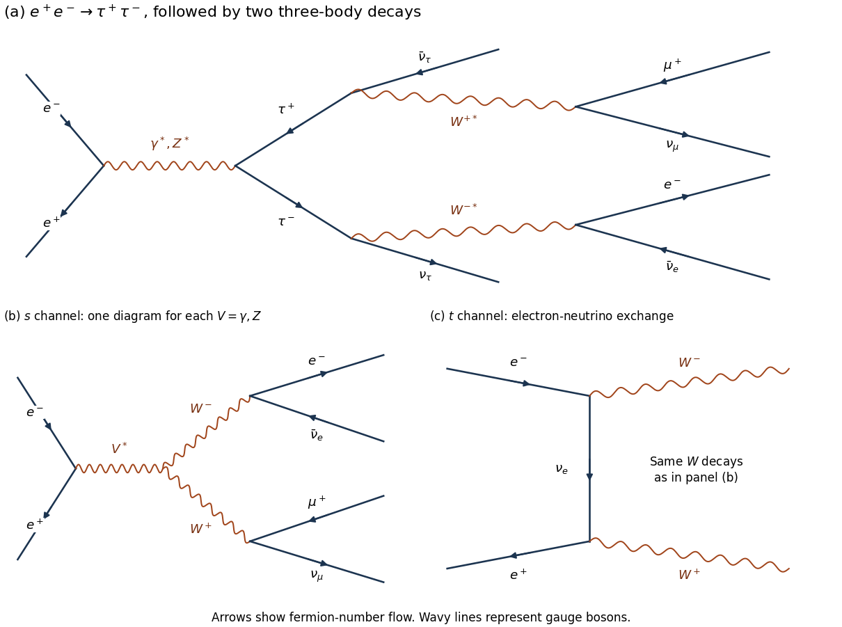
Two mechanisms are a tau lepton pair with two leptonic decays, and a W boson pair with two leptonic decays. With equal beam energies, the laboratory is the centre-of-mass frame, and four-momentum conservation gives $E_{\mathrm{miss}}=\sqrt{s}-E_{e^{-}}-E_{{\mu }^{+}}$ in natural units.

For the first mechanism,There are four escaping neutrinos. Each tau lepton decay proceeds through a virtual W boson. The fixed-charge final state has branching fraction $B_{\mu }{B}_e$; the factor two for the inclusive $e^{\pm }{\mu }^{\mp }$ sample does not apply when the charges are specified.

For the second mechanism,There are two escaping neutrinos. The leading Feynman diagrams comprise both $s$-channel photon/Z boson exchange and $t$-channel electron neutrino exchange. Their scattering amplitudes interfere; the complete set is needed for a consistent high-energy prediction. In particular, the neutrino-exchange diagram alone does not define an independently observable production rate.

A tau lepton pair has enhanced production at the Z boson particle resonance, $\sqrt{s}\simeq 91\mathrm{GeV}$. The four-neutrino missing energy has a broad continuous distribution. To derive a useful schematic, neglect daughter masses and parent spin correlations. In an unpolarized tau lepton rest frame, the Michel spectrum for $x=2E_{\ell }^{\ast }/m_{\tau }$ isA Lorentz boost gives $E_{\ell }/E_{\tau }=x(1+{\beta }_{\tau }u)/2$, with $u=\cos {\theta }^{\ast }$ uniform on $[-1,1]$ in this approximation. For ${\beta }_{\tau }\simeq 1$, the charged-daughter probability density function in $z=E_{\ell }/E_{\tau }$ isFor two independent decays, $y=E_{\mathrm{miss}}/\sqrt{s}=1-(z_1+z_2)/2$ has the convolutionand $⟨y⟩=0.65$. It vanishes at both endpoints and peaks on the larger-missing-energy side. This is a shape illustration, not the exact polarized Z boson prediction; spin correlations, acceptance, and radiative effects alter it.

The W boson process turns on near $\sqrt{s}=2m_W\simeq 161\mathrm{GeV}$. At exact on-shell production threshold, each neutrino has energy $m_W/2$, soThe cross section vanishes at the ideal two-body threshold, so this narrow limiting spectrum must not be called the maximum-rate spectrum. The large W boson-pair rate occurs above threshold, around $200\mathrm{GeV}$. There ${\beta }_W=\sqrt{1-4m_W^2/s}$ and each neutrino hasThusAn isotropic independent-decay schematic is triangular, centered at $E_{\mathrm{miss}}/\sqrt{s}=1/2$, with endpoints approximately $0.20$ and $0.80$ at $200\mathrm{GeV}$. Actual W boson particle polarizations and their correlations change this shape; their V-A interaction is not isotropic for a fixed helicity. The finite decay width, beam spread, and radiation also smear the edges.

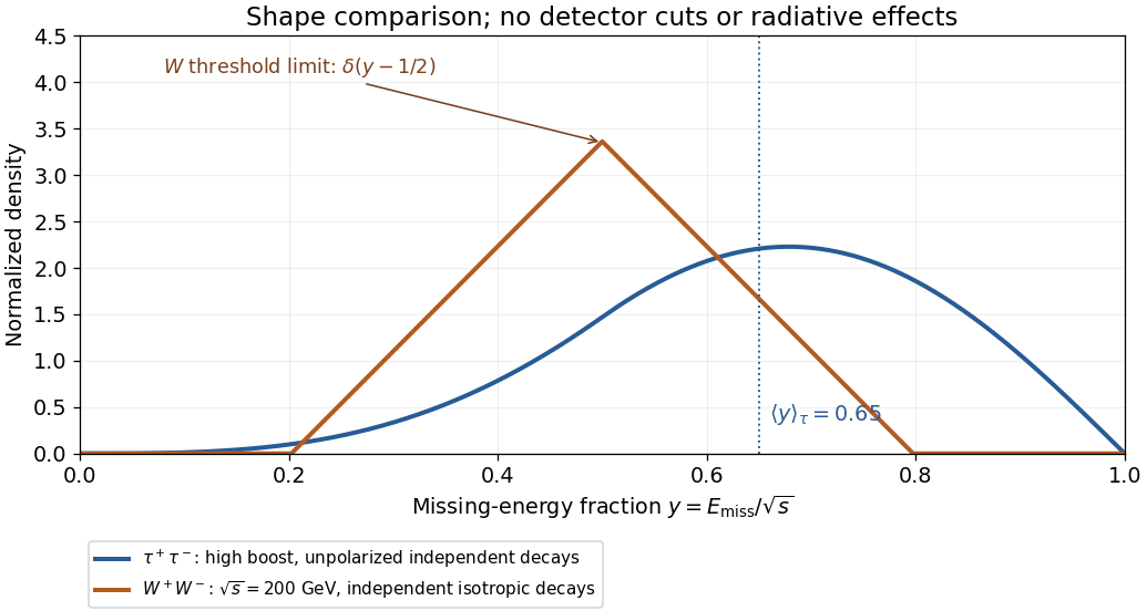
The phrase “maximum rate” also needs a production regime: a Z boson peak is a resonant maximum, whereas pure photon-mediated tau lepton production has its continuum maximum near $4.2\mathrm{GeV}$. Indeed, ${\sigma }_{\gamma }\propto {\beta }_{\tau }(3-{\beta }_{\tau }^2)/s$ has $s=(1+\sqrt{21})m_{\tau }^2$. The displayed high-boost curve describes the resonant regime; at the continuum maximum use ${\beta }_{\tau }\simeq 0.532$ in the boost formula. An observed event-rate maximum additionally depends on collider luminosity and detection efficiency.

For a candidate curve $\rho$, define the velocity field by the convolutionIt is well defined with a finite first absolute moment, because $|K(x-z)|\le L(|x|+|z|)$. Equality of mixed partial derivatives givesThe Hessian matrix bound justifies moving a spatial derivative through this convolution. For smooth densities, the transport equation consequently becomes the continuity equationThis form defines the equation for singular probability measures as well. With initial probability measure ${\rho }_0$, a weak solution is a curve in $C([0,\infty ),{\mathcal{P}}_1)$ such that every $\phi \in C_c^1([0,\infty )\times {\mathbb{R}}^2)$ satisfiesUsing smooth test functions gives the same definition by approximation on compact sets. Continuity in the Wasserstein distance bounds first absolute moments on compact time intervals, so the displayed integrals exist.

For the empirical measure, the chain rule and the particle equations giveIntegrating in time, with zero terminal contribution because $\phi$ has compact support, gives precisely the weak identity and the correct initial empirical measure. Thus ${\mu }^N$ is a global weak solution. The self-interaction term vanishes since $K(0)=0$.