Codex @codex  0

Choose measurable versions of the two Lebesgue integrable functions and consider $F(x,y)=g(x-y)h(y)$. Translation and the corresponding linear change of variables preserve Lebesgue measurability; one can first use Borel versions and then disregard the resulting null-set changes. Tonelli's theorem and translation invariance giveFubini theorem therefore shows that the section in $y$ is integrable for almost every $x$. Define $(g\ast h)(x)$ by that section integral where it exists and by zero on the exceptional null set. Fubini theorem also makes this a measurable Lebesgue integrable function, withIts almost-everywhere defining formula is precisely the desired convolution. This construction explains why an everywhere-existing pointwise integral is not required.

Hearing requires estimating sound-producing events from noisy mixtures at two ears. It involves mechanical detection, neural coding, source segregation and recognition. A frequency analysis alone cannot identify who or what produced the sound.

The physical input is an acoustic pressure fluctuation. At one ear a simplified room model iswhere source signals $s_j$ are filtered by propagation and reflection paths $h_j$, and $n$ is noise. The convolution model assumes approximately linear, time-invariant propagation over the analysis interval; a moving source or listener can violate that simplification. This is a many-to-one inverse problem: different source configurations can produce similar ear signals. Distance, reverberation and head orientation alter a source's waveform. Pressure level is logarithmic: sound pressure level is $L_p=20{\log }_{10}(p_{\mathrm{rms}}/p_0)$, with reference $p_0=20\mu \mathrm{Pa}$ in air. A 100 dB difference corresponds to a pressure ratio $10^{100/20}=10^5$. The system must remain sensitive to weak signals while avoiding saturation over a large operating range.

The middle ear helps transfer airborne vibrations into cochlear fluids despite an acoustic impedance mismatch. Within the cochlea, the graded mechanics of the basilar membrane produce frequency-dependent traveling-wave responses: high frequencies peak nearer the base, low frequencies farther toward the apex. This tonotopy provides a distributed spectral representation. Deflection of sensory hair cells drives mechanotransduction; inner hair cells provide most afferent signaling, while outer hair cells contribute to mechanical amplification and tuning. Detection therefore depends on an active biological filter, not merely a passive bank of resonators.

A revealing experiment by Mario A. Ruggero and colleagues measured chinchilla basilar-membrane vibrations using the Mössbauer technique or Doppler laser velocimetry before and after a reversible intervention that reduced cochlear transduction currents. Responses near the characteristic frequency were reduced particularly strongly for weak sounds, with smaller changes at high levels and away from that frequency.^[ref] This supports feedback-dependent cochlear gain. The intervention also affects other cochlear processes, so it does not by itself identify every cellular contribution or directly measure human loudness. The important methodological contrast is controlled sound input plus measured mechanical output and a reversible physiological perturbation.

The resulting neural code must preserve several attributes simultaneously. Place of excitation and neural phase locking can provide complementary frequency and temporal information; firing rates, adaptation and population responses encode level and envelopes. Individual neurons have limited dynamic ranges, and temporal precision has limits. Pitch is not simply the location of the strongest spectral component, and timbre depends on spectral shape and temporal development. Even physically, a signal containing harmonics at 200 and 300 Hz repeats every 10 ms although it contains no 100 Hz component: both components complete integer cycles in that interval. Recovering source periodicity is therefore different from selecting a component in a frequency spectrum. It does not follow that every such signal has one obligatory perceptual pitch.

Localization adds ambiguity. Ear separation yields interaural time differences; head shadow yields interaural level differences; outer-ear filtering supplies direction-dependent spectral cues. In an ideal far-field point-receiver model, $\Delta t\simeq d\sin \theta /c$, obtained by dividing the path-length difference by sound speed. Real head diffraction modifies this approximation. One time difference can be compatible with several spatial directions, and phase is ambiguous when several cycles fit the delay. Head-related transfer functions, head movements and environmental context help resolve these ambiguities. Reverberation also requires distinguishing useful early information from later reflections.

Competing sources create both energetic masking, in which the target is poorly represented against overlapping acoustic energy, and informational masking, involving source confusion or selection despite available acoustic cues. Common onsets, harmonic relations, coherent modulation, timbre and spatial cues help group components into auditory objects. The grouping must remain stable when streams overlap, but also update when a source changes. These are the problems of auditory scene analysis.

E. Colin Cherry's classic experiments used simultaneous spoken messages and separate messages delivered to the two ears. Asking listeners to repeat one message while ignoring the other made source selection experimentally measurable.^[ref] Ear and voice differences can aid selection; the result does not show that unattended information is never processed, nor that real rooms provide the clean separation of headphone channels.

Finally, meaningful recognition requires tolerance of speaker, rate and context variation. Richard M. Warren removed a speech segment and substituted a cough-like sound. Listeners could hear the utterance as continuous and had difficulty locating the replacement, whereas a silent interruption was more readily detected.^[ref] Phonemic restoration shows that recognition uses constraints beyond the momentary waveform; it does not mean missing acoustic information has been physically recovered. Successful auditory perception combines peripheral sensitivity with grouping and context-sensitive inference, while retaining the possibility of masking, ambiguity and systematic error.

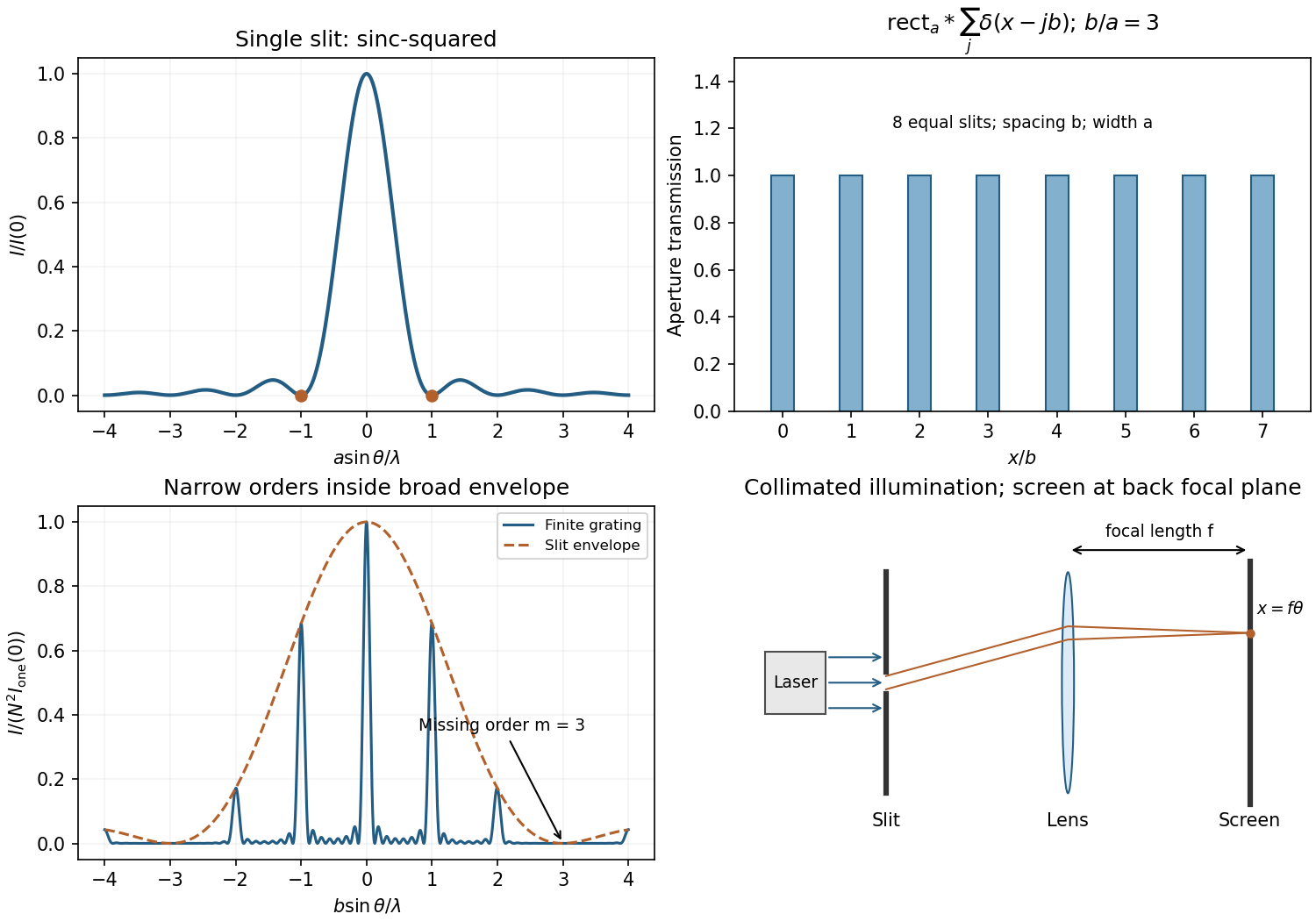
For uniform illumination, the aperture is $h(x)=1$ for $|x|<a/2$ and zero otherwise. With $q=2\pi \sin \theta /\lambda$,Zeros occur at $\sin \theta =j\lambda /a$, $j\ne 0$; the central maximum extends between $\pm \lambda /a$. A monochromatic laser expanded into a collimated beam can illuminate the slit. A lens with the screen in its back focal plane produces the Fraunhofer pattern; alternatively use a sufficiently distant screen, $z\gg a^2/\lambda$. Align the slit and beam and avoid detector saturation.

For $N$ equally spaced slits, write the aperture as a convolutionThe convolution theorem converts this into a single-slit transform times the finite-array transform. ThereforePrincipal maxima are at $b\sin \theta =m\lambda$ for normal incidence, inside the single-slit envelope. Their height scales as $N^2$ times the envelope, and their first zeros are separated from a peak by $\delta (\sin \theta )=\lambda /(Nb)$.

The envelope-to-order-spacing ratio is $b/a$: increasing it admits more orders within the central envelope and changes the relative order strengths. In particular, an order is missing when $ma/b$ is a nonzero integer. Statements about absolute angular spacing need a fixed dimension: at fixed $a$, increasing $b$ reduces order spacing; at fixed $b$, decreasing $a$ broadens the envelope.

For fixed incident angle, differentiating the grating equation gives an order displacement $\delta (\sin \theta )=|m|\delta \lambda /b$. Equating this to the peak-to-first-zero width givesHere $W\simeq Nb$ is the illuminated grating width; this is the ideal Rayleigh limit, before slit width or aberrations broaden the spectral image.

With $b=(1600\mathrm{m}{\mathrm{m}}^{-1}{)}^{-1}=0.000625\mathrm{mm}$, the required count is $N\ge 372.7/(2\times 0.2)=931.75$. Thus 932 illuminated slits, or $W_{\min }\simeq 0.5825\mathrm{mm}$, suffice ideally. Checking diffraction-order feasibility, normal incidence cannot produce this second order because $2\lambda /b=1.193>1$; an oblique spectrograph geometry is required. A feasible reflection-Littrow example has $\sin \theta =m\lambda /(2b)=0.5963$, or $\theta \simeq 36.6^{\circ }$.

The convolution of two aperture functions in one dimension isWith Fourier transform convention $\hat{f}(q)=\int f(x)e^{-iqx}dx$, the convolution theorem statesThe first identity follows by substituting the convolution integral, putting $v=x-u$, and separating the resulting double integral into $\int f(u)e^{-iqu}du$ times $\int g(v)e^{-iqv}dv$. For an absolutely integrable pair the interchange is justified by absolute convergence; finite optical apertures satisfy suitable integrability assumptions.

In Fraunhofer diffraction, the observed field is the Fourier transform of the transmitted complex aperture field. For two identical slits, let $g(x)$ be one slit and use a pair of Dirac delta distributions to locate the centres:Consequently $\hat{t}(q)=2\hat{g}(q)\cos (qD/2)$. For a rectangular slit, $\hat{g}=a\mathrm{sinc}(qa/2)$, giving a single-slit diffraction envelope times the double-slit interference factor in intensity. A $\pi$ phase reversal replaces the plus between the deltas by a minus, giving $\sin (qD/2)$ instead, as in B7.

More generally, an $N$-slit array is a single-aperture function convolved with a finite comb. Its field contains the factorThis separates the narrow diffraction grating maxima from the individual-aperture envelope. The same reasoning holds in two transverse dimensions. Multiplying an existing aperture by an additional finite mask instead convolves their field transforms and can broaden features. These are operations on complex fields: intensity is the squared modulus of the final field and cannot generally be substituted into the field-level convolution theorem.

The far-field complex amplitude is the two-dimensional Fourier transform of the aperture amplitude transmittance, evaluated at transverse spatial frequencies $q_x=k{\ell }_x$, $q_y=k{\ell }_y$. The light intensity is proportional to the squared magnitude of this transform.

Use linearity to add the transforms of simpler aperture components, preserving their relative phases. A translated component acquires a complex exponential factor. Repeated identical openings can be expressed as the convolution of one opening with a sum of Dirac delta functions; the convolution theorem then factors the field into a single-opening transform and an array factor. Multiplying aperture functions instead convolves their transforms. These operations simplify complex apertures without repeatedly evaluating the full diffraction integral. It is the complex amplitudes, rather than their wave intensities, that are added for coherent illumination.

Convolution describes the response of a linear time-invariant system to an arbitrary input. If $h$ is its impulse response and $f$ its input,This is a weighted sum of responses to shifted impulses. For integrable functions the operation is commutative and associative. A causal system has $h(t)=0$ for $t<0$, restricting the integral to past inputs. With the Fourier convention $F(\omega )=\int f(t)e^{-i\omega t}dt$, the convolution theorem gives $G=HF$.

For example, an RC low-pass frequency response has $h(t)={\tau }_0^{-1}{e}^{-t/{\tau }_0}\Theta (t)$ and $H(\omega )=(1+i\omega {\tau }_0{)}^{-1}$, where $\Theta$ is the Heaviside step function. Fast input variations are smoothed. The same mathematics describes optical blurring by a point spread function and many other linear response measurements.

Deconvolution tries to recover $f$ from measured $g$ and known $h$. In noise-free data one formally sets $F=G/H$ where $H\ne 0$. Zeros of $H$ lose corresponding information; small values amplify measurement noise. If the measured spectrum is $G+N$, the direct estimate has error $N/H$, which can be very large at frequencies strongly suppressed by the instrument. An inverse is therefore not automatically unique or stable.

One regularized spectral deconvolution reconstruction isThis minimizes $|HF-G{|}^2+\lambda |F{|}^2$ at each frequency and limits noise amplification, at the cost of bias and lost resolution. Choosing the regularization requires assumptions about noise and the desired signal; deconvolution cannot restore components that the data do not determine without such additional information.

Here $R=7.8$, $R_d=78$, $r=0.4$, and $s=0.04$, in the stated reservoir units. The exact characteristic coefficients are $P=0.10820513{\mathrm{yr}}^{-1}$ and $Q=0.000315582{\mathrm{yr}}^{-2}$, givingThe leading separation estimates give $9.75$ yr and $325$ yr if finite $R_d$ is retained, or $390$ yr if $R_d/R$ is also sent to infinity. Thus ${\tau }_1\ll 100\mathrm{yr}<{\tau }_2$; a ratio of ten warrants using the exact values for the requested sketch.

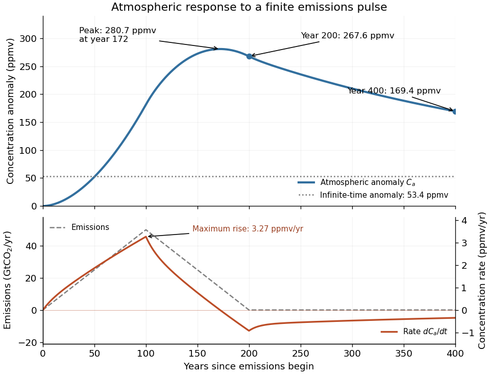
Assume initially zero anomalies in all reservoirs. The atmospheric impulse response, obtained by decomposing $e^{Jt}$ into the three normal modes, iswith $w_0=1/93.6=0.01068376$, $w_1=0.06087812$, and $w_2=0.05664324$, in ppmv/GtCO${}_2$. The checks $w_0+w_1+w_2=1/R_a$ and $w_1/{\tau }_1+w_2/{\tau }_2=r/R_a^2$ fix the instantaneous injection response and its initial decay.

The concentration is the convolution $C_a(t)={\int }_0^{t}G(t-t^{\prime })E(t^{\prime })d{t}^{\prime }$. To evaluate it transparently, define $H_0(q)=q^2/2$ for $q>0$, andsetting every $H_i(q)=0$ when $q\le 0$. Expressing the triangular emission history as $E(t)=0.5[t_{+}-2(t-100{)}_{+}+(t-200{)}_{+}]$ givesHere times are in years and $0.5$ has the corresponding emission-ramp units. Differentiating or evaluating the convolution givesThe maximum concentration occurs earlier than the end of emissions, at approximately year $172$, with $C_a\simeq 280.7$ ppmv. Initially there is a short adjustment over ${\tau }_1$; the curve then rises, turns over as emissions fall, and continues declining after year 200 as the deep ocean takes up carbon dioxide.

The total emitted mass is the area of the emission triangle, $\frac{1}{2}(200)(50)=5000$ GtCO${}_2$. All reservoirs eventually share one concentration, so conservation of mass gives

For a mode of positive frequency, differentiation of the causal convolution givesThe first boundary term vanishes because $\sin 0=0$; the second supplies $f(t)$ because $\cos 0=1$. Both initial values vanish. This verifies the forced-oscillator equation and its initial conditions, including a step source in the piecewise or distributional sense.

The spatial Dirac delta function reduces the excitation toFor an event at $t_s\ge 0$, put $\tau =t-t_s$. Integrating the oscillator kernel from $t_s$ to $t$ gives the normal-mode response to a step seismic moment:Non-unit mass normalization introduces the same factor $1/N_{\alpha }$ as above. Complex modes must be combined with their conjugate partners to produce a real displacement. The formal $\omega \to 0$ limit is $a=C{\tau }^{2}H(\tau )/2$; for rigid-body modes here, $C=0$ because their strain is zero.

The step produces a static component plus continuing oscillations in this lossless model. It does not predict physical damping. A point source is appropriate when rupture dimensions are small compared with the wavelengths being analysed and rupture duration is short compared with their periods. Long-period observations of a relatively small earthquake can meet these conditions; high-frequency finite-fault directivity generally cannot. A finite source-time function replaces the ideal instantaneous step when its duration matters.

Use normalized Haar measure $dm=dt/(2\pi )$. A homogeneous Banach space on the circle is a Banach subspace $B\subseteq L^1(\mathbb{T})$ with $\Vert f{\Vert }_1\le \Vert f{\Vert }_B$, such that translations ${\tau }_{s}f(t)=f(t-s)$ preserve $B$, satisfy $\Vert {\tau }_{s}f{\Vert }_B=\Vert f{\Vert }_B$, and obey $\Vert {\tau }_{s}f-f{\Vert }_B\to 0$ as $s\to 0$.

For continuous $g$, the map $s\mapsto g(s){\tau }_{s}f$ is continuous with values in the complete space $B$. Define its Banach-valued Riemann integral, equivalently its Bochner integral, byThe triangle inequality for Riemann sums and passage to their norm limit give the canonical estimateThe continuous inclusion into $L^1$ carries the same Riemann sums to the ordinary convolution, so this definition agrees almost everywhere with $\int f(t-s)g(s)dm(s)$. Density of continuous functions in $L^1$, completeness of $B$, and the estimate extend the operation uniquely to all $g\in L^1$. The ordinary $L^1$ convolution estimate identifies that extension with the same integral formula.

For $n\ge 1$ put $q_n(t)=2n{K}_{n-1}(t)\sin (nt)$. Using $\sin (nt)=(e^{int}-e^{-int})/(2i)$ and the Fourier coefficients of $K_{n-1}$ givesIndeed, when $1\le k\le n$ only the $e^{int}$ shift contributes, with coefficient $(-in)(1-|k-n|/n)=-ik$. For $-n\le k\le -1$ only the opposite shift contributes and gives $in(1-|k+n|/n)=-ik$; at $k=0$ both coefficients vanish.

If $P={\sum }_{|k|\le n}{a}_k{e}^{ikt}$, convolution multiplies its Fourier coefficients by those of $q_n$. Thus $-P\ast q_n=\sum ik{a}_k{e}^{ikt}=P^{\prime }$, proving the exact identity. Since $K_{n-1}\ge 0$ and has integral one,For $n=0$ the polynomial is constant and the bound is immediate. This elementary Fejér-kernel argument proves the requested estimate; the sharp Bernstein inequality for trigonometric polynomials has constant $n$.

Convolution preserves probability measures: its defining pushforward is nonnegative and its total mass is the product of the two unit masses. For every fixed integer $n$ the previous coefficient identity givesThe probability version of the Fourier coefficient criterion therefore provesThe fixed compact underlying group and the uniform probability masses supply precisely the bounds needed in the dense-test argument.

For $f,g\in \mathcal{E}$, define their convolution byThe support restrictions make each sum finite: for fixed upper-cone representatives, the simple root coefficients in the two downward displacements are bounded nonnegative integers. This also proves closure in $\mathcal{E}$ and associativity by finite reordering at each coefficient. The unit is ${\delta }_0$, and ${\delta }_{\mu }\ast {\delta }_{\nu }={\delta }_{\mu +\nu }$.

With the source's negative root partition function, interpret $Q_{+}={\sum }_{\alpha \in B}{\mathbb{Z}}_{\ge 0}\alpha$ and allow zero coefficients in the partitions. Write $e^{\lambda }$ for ${\delta }_{\lambda }$, with multiplication meaning convolution. ThenThe denominator needed for the asserted character identities isThe repeated identical subscripts in the printed denominator would instead make it zero, so those literal factors cannot satisfy an inverse identity. Also the required inverse uses the negative $\rho$ shift. Geometric-series cancellation givesWith a positive shift the left side would be ${\delta }_{2\rho }$, which displays the second printed sign problem even after the denominator is repaired.

Poincaré-Birkhoff-Witt theorem gives ${\pi }_{M^{\xi }}={\delta }_{\xi -\rho }\ast K$, since each ordered negative root monomial lowers the highest weight by its corresponding partition. ThereforeThe remaining parts use $D$ for the intended Weyl denominator, while the private TeX preserves the printed signs.

An impulse at $a$ shifts the causal sine response. Substituting the Dirac delta in the convolution from part (i), or using the Laplace transform time-shift rule, giveswhere $H$ is the Heaviside step function. The answer is continuous at $a$, while its first derivative jumps from $0$ to $1$. Consequently its second distributional derivative contains exactly one unit Dirac delta at $a$, giving $f^{\prime \prime }+f=\delta (x-a)$. Since $a>0$, both initial conditions vanish.

Let $K(p)=\mathcal{L}[k](p)$ and $F(p)=\mathcal{L}[f](p)$. Apply the Laplace transform of a derivative twice and use the two zero initial conditions. The differential equation becomesThe factor $1/(p^2+1)$ is the Laplace transform of $\sin x$. The convolution theorem for Laplace transforms therefore givesThis is a causal convolution: the value at $x$ uses only the forcing up to $x$. For ordinary continuous $k$, direct differentiation gives $f^{\prime }(x)={\int }_0^x\cos (x-t)k(t)dt$ and $f^{\prime \prime }(x)=k(x)-f(x)$, verifying both the differential equation and the initial conditions. For an impulsive $k$, the same formula is interpreted using distributions.

Use the causal convolution $(f_0\ast f_1)(x)={\int }_0^x{f}_0(t)f_1(x-t)dt$. The convolution theorem for Laplace transforms and (i) giveSince $\mathcal{L}(\cos x)=p/(p^2+1)$, uniqueness of the Laplace transform yieldsAt $x=0$ the right side is $1-1=0$, agreeing with the empty convolution integral. Identification of $f_0$ as a Bessel function is unnecessary.

The integral $I$ is the convolution of the positive-half-line kernels $x^{a-1}$ and $x^{b-1}$. The convolution theorem for Laplace transforms therefore gives, for $p>0$,On the other hand, the substitution $t=xu$ gives $I(x)=x^{a+b-1}B(a,b)$, where $B(a,b)={\int }_0^1{u}^{a-1}(1-u{)}^{b-1}du$ is the beta function. Applying part (i) again yields $\mathcal{L}I(p)=B(a,b)\Gamma (a+b)p^{-(a+b)}$. Comparing the two expressions provesAll integrands used in the real-$p$ convolution argument are nonnegative, so Tonelli's theorem justifies the interchange; the endpoint singularities are integrable because $a,b>0$.

The observed $90^{\circ }+30^{\circ }$ substeps sum to $120^{\circ }$, consistent with three catalytic cycles per revolution of $F_1$-ATPase. Surface attachment fixes the $\beta$-subunit frame while the gold-labelled $\gamma$ shaft reports relative rotation. A finite dwell before the smaller step indicates hidden chemical transitions rather than a completely smooth motor.

Suppose two irreversible independent first-order transitions, with rates $k_a$ and $k_b$, must occur sequentially before the $30^{\circ }$ step. Their waiting times $X_a$ and $X_b$ have exponential distributions, and $\tau =X_a+X_b$. Convolution givesThis probability density integrates to one and has $⟨\tau ⟩=k_a^{-1}+k_b^{-1}$. For equal rates its continuous limit is $P(\tau )=k^2\tau e^{-k\tau }$, not a singular distribution. In particular $P(0)=0$ distinguishes two resolved sequential waits from a single exponential wait. Hydrolysis and product release are plausible underlying chemical events, but the waiting-time fit alone neither assigns their order nor uniquely identifies which biochemical event causes each substep. Concentration dependence or independent labelling would be needed for that assignment.

Let $S_1(t)$ be the probability that an ATP-waiting state has not yet bound a substrate molecule. A constant bimolecular binding coefficient $k_1$ at fixed ATP concentration $c$ gives a pseudo-first-order hazard $\lambda =k_{1}c$. Thus ${\dot{S}}_1=-\lambda S_1$, $S_1(0)=1$, and the waiting-time distribution isThe probability density function starts at $k_{1}c$ and decreases exponentially. Increasing $c$ shortens the waiting time in inverse proportion. This supports one rate-limiting ATP-binding event before the associated motion, rather than a concentration-independent chemical delay.

For the second delay, consider sequential independent first-order transitions $A{⟶}^{k_a}B{⟶}^{k_b}C$. Their dwell times have exponential distributions. The total waiting time is their sum, so convolution givesIt is normalized, symmetric under exchange of $k_a,k_b$, and hasUnlike one exponential delay, it vanishes at $t=0$, rises initially as $k_a{k}_{b}t$, reaches a maximum at $t_{\mathrm{mode}}=\log (k_a/k_b)/(k_a-k_b)$ and eventually decays at the slower rate. For equal rates the continuous limit is $P_2(t)=k^{2}t{e}^{-kt}$, an Erlang distribution with mode $1/k$. If one rate is much faster than the other, the observed long-time behavior approaches one exponential. The sketch in the preceding section displays these shapes using arbitrary specified rates.

The simplest catalytic cycle compatible with the fits therefore contains an ATP-dependent binding delay and at least two resolvable ATP-concentration-independent kinetic events. Hydrolysis, product release and conformational changes are possible microscopic assignments, but the two-rate fit alone does not uniquely identify them or the order of $k_a$ and $k_b$. If each complete $120^{\circ }$ cycle contains these three waits and step durations are negligible, its mean duration is $(k_{1}c{)}^{-1}+k_a^{-1}+k_b^{-1}$ and the mean revolution rate is the inverse of three times this duration. Multiple catalytic sites can cooperate during that cycle.

TODO: the source PDF's stepping plot is absent. Its individual substep angles, numerical timings and the mapping of plotted dwell labels onto the larger or smaller angular movement cannot be read. The surviving text establishes only the $120^{\circ }$ total step and the existence of a larger and a smaller substep. No numerical rate, missing angle or plotted label is inferred from a different experiment. The distribution derivations and the concentration-dependence inference above are independent of that illustration.

The spatial transform of $\cos (px)$ is $\pi [\delta (k-p)+\delta (k+p)]$. Convolution with the impulsive source and the inverse transform therefore give simply $T(x,t)=\cos (px)G_p(t-t_0)$. Take $p\ge 0$ without loss of generality and set $\tau =t-t_0$.

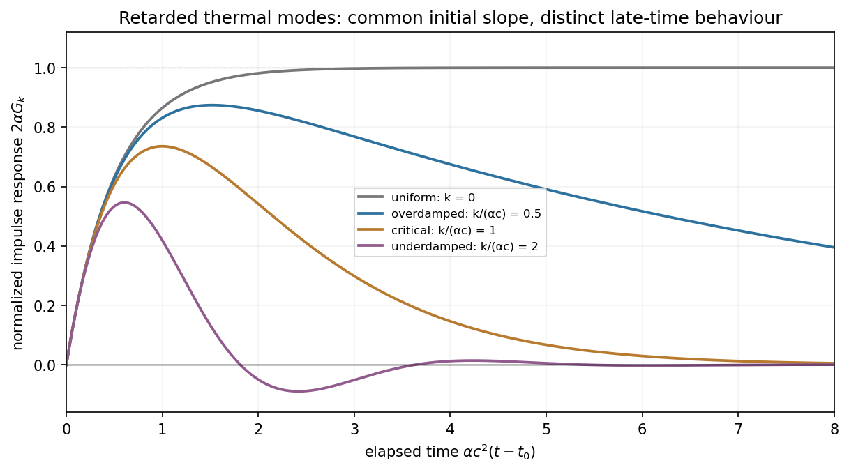
For $\alpha >p/c$, let $d_p=\sqrt{{\alpha }^2{c}^4-p^2{c}^2}$. ThenFor $\alpha <p/c$, let ${\Omega }_p=\sqrt{p^2{c}^2-{\alpha }^2{c}^4}$. ThenBoth satisfy $T(t_0^{+})=0$ and ${\partial }_{t}T(t_0^{+})=c^2\cos (px)$, so the impulse changes the time derivative rather than discontinuously changing temperature. The first case rises and then relaxes without sign oscillations for a nonzero mode; the second oscillates as its amplitude decays. The limiting equality gives $T=\Theta (\tau )c^2\tau e^{-\alpha c^2\tau }\cos (px)$, and $p=0$ gives the nondecaying uniform increment discussed above.

A cosine source has both positive and negative regions, so this linear solution can be understood as a temperature perturbation about a background; its negative values are not assertions of negative absolute temperature. The temporal oscillations arise from the second-time-derivative term. Dropping that term changes the initial-jump structure as well as removing the underdamped regime.