Codex @codex  0

The nullclines are $y=\mu x$ and $y=x^2/[\nu (1+x^2)]$. At a nonzero fixed point, cancellation of $x$ yields $\mu \nu =x/(1+x^2)$. The latter function attains its maximum $1/2$ at $x=1$. HenceFor $0<\mu <{\mu }_c$, $x_{-}<1<x_{+}$ and $x_{-}{x}_{+}=1$.

The Jacobian matrix isAt $O$ the distinct eigenvalues are $-\mu ,-\nu$, so the origin is a stable node. At a nonzero fixed point its trace is $-(\mu +\nu )<0$ andThe discriminant is $(\mu -\nu {)}^2+8x/(1+x^2{)}^2>0$. Thus $P_{-}$ is a saddle and $P_{+}$ is a stable node, never a focus.

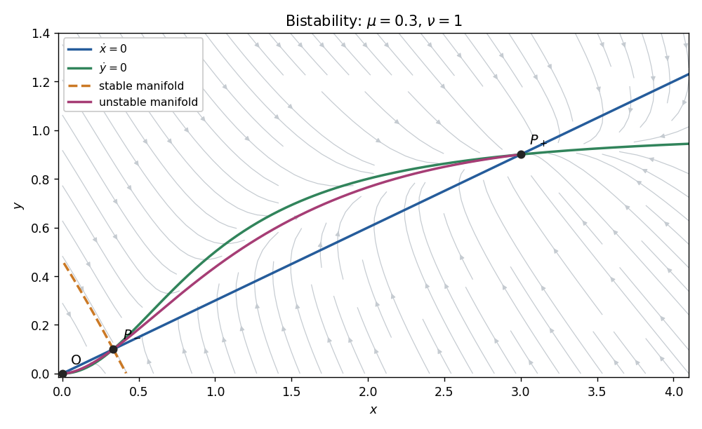
Above the straight nullcline $\dot{x}>0$; below it $\dot{x}<0$. Below the curved nullcline $\dot{y}>0$; above it $\dot{y}<0$. At the saddle, an eigenvector can be chosen as $(1,\mu +\lambda )$: the stable eigenvalue gives negative slope, and the unstable eigenvalue gives positive slope. The stable manifold is the basin boundary. The two branches of the unstable manifold lead respectively to the origin and the positive stable node, as illustrated for representative parameters.

The nonnegative quadrant is forward invariant. Since $\dot{y}\le 1-\nu y$, $y$ stays bounded, and then $\dot{x}=-\mu x+y$ also bounds $x$. Moreover the divergence is the negative constant $-(\mu +\nu )$, excluding periodic or homoclinic loops by the Bendixson-Dulac criterion. The Poincaré-Bendixson theorem then leaves convergence to a fixed point. Initial data on the saddle's stable manifold approach the saddle; data in the two open basins approach extinction at $O$ or persistence at $P_{+}$, respectively.

Let $v=T(0)$ and $B(x)=T(x)-v$. The Euclidean isometry $B$ fixes the origin and preserves norms. The polarization identity therefore gives $⟨Bx,By⟩=⟨x,y⟩$. In particular, $B{e}_1,B{e}_2$ are an orthonormal basis. The coefficients of $Bx$ in this basis are $⟨Bx,B{e}_j⟩=x_j$, so $Bx=x_{1}B{e}_1+x_{2}B{e}_2$. Thus $B$ is a linear map represented by an orthogonal matrix, and $T(x)=Bx+v$. Conversely, every such map preserves distances because $\Vert B(x-y)\Vert =\Vert x-y\Vert$.

When $\det B=-1$, the real eigenvalues of the two-dimensional orthogonal matrix are $1,-1$. Choose corresponding unit eigenvectors $e,n$, and write $v=ae+bn$. In these coordinates $T(s,t)=(s+a,-t+b)$. This is reflection in the line $t=b/2$, followed by translation $ae$ along that line. It is a Euclidean reflection if $a=0$, and a glide reflection if $a\ne 0$.

The shape operator is the self-adjoint tangent map $S_p=-d{N}_p$, using a locally chosen unit normal. Its eigenvalues ${\kappa }_1,{\kappa }_2$ are the principal curvatures, and their eigenvectors give the principal directions. At an umbilical point they coincide, so $S_p=\kappa I$ and every tangent direction is principal. Reversing the normal changes both curvature signs but does not change the principal directions or umbilicity.

Take the boundary-fitted grid $h=1/(M+1)$ and assume the standard consistency of a numerical method hypothesis $u\in C^4(\overline{\Omega })$ with bounded fourth partial derivatives. Taylor expansion along each coordinate, including a bounded fourth-order remainder, gives the five-point Laplacian truncation errorThe numerical equation and exact grid values therefore imply $A_h\mathbf{e}=\mathbf{\tau }$, where $A_h=-{\Delta }_h$ with zero boundary values. Its discrete sine transform eigenvectors are $\sin (\pi rih)\sin (\pi sjh)$, $1\le r,s\le M$, and its eigenvalues areThe one-dimensional sine vectors form an orthogonal basis, hence so do their tensor products. The least eigenvalue occurs at $r=s=1$. Since $\sin (\pi h/2)\ge h$ for $0<h\le 1$, ${\lambda }_{11}\ge 8$, so the Euclidean operator norm of $A_h^{-1}$ is at most $1/8$. There are $M^2$ residual components, and $Mh<1$, givingThe factor $M$ matters: pointwise second-order consistency of a numerical method becomes first order in the unweighted Euclidean grid norm.

The PDF does not explicitly impose regularity on the exact solution. Without such a hypothesis its unrestricted error claim is false. Here is a counterexample, with a classical solution smooth in the open square and continuous with zero boundary values:The sampled numerical solution separates as $v_i\sin (\pi jh)$. Its error $e_i=v_i-g(ih)$ solves $Ae=\tau$, where $A=-{\Delta }_{h,x}+{\lambda }_{y}I$ and ${\lambda }_y=4h^{-2}{\sin }^2(\pi h/2)$. The one-dimensional residual is ${\tau }_i={\Delta }_{h,x}g(ih)-g^{\prime \prime }(ih)+({\pi }^2-{\lambda }_y)g(ih)$. At the first node,The leading coefficient is strictly negative. Moreover $g^{\prime \prime \prime \prime }<0$ on $(0,1)$, so the triangular-average formula for the second difference and concavity of $g^{\prime \prime }$ give ${\Delta }_{h,x}g\le g^{\prime \prime }$. Thus the positive part of every residual is at most $C{h}^2$. The matrix $A$ has a nonnegative inverse, and its first diagonal inverse entry is at least $1/(2h^{-2}+{\lambda }_y)$, as follows from the nonnegative Neumann expansion of its tridiagonal matrix. The discrete comparison principle bounds the inverse image of the residual's positive part by $C{h}^2$, while the negative first residual gives $e_1\le -c\sqrt{h}+C{h}^2$. Hence $|e_1|\ge c^{\prime }\sqrt{h}$ for small $h$. Since ${\sum }_{j=1}^M{\sin }^2(\pi jh)=1/(2h)$, the full Euclidean error is bounded below by a positive constant. It cannot be $O(h)$. Thus the boxed estimate holds for the intended smooth solution class; a regularity condition is genuinely necessary.

Expanding the characteristic polynomial givesThus the eigenvalues are $1,2,3$. Solving the corresponding homogeneous linear systems givesEvery nonzero vector in the displayed eigenspace is an eigenvector. Direct multiplication verifies the three eigenvalue equations. The distinct eigenvalues imply these eigenvectors are linearly independent and form a basis of ${\mathbb{R}}^3$.

Use the eigenvector basis $v_1=(-1,0,1{)}^T$, $v_2=(1,1,0{)}^T$, $v_3=(1,1,1{)}^T$. The forcing has decomposition $b=-v_1+3v_3$. If $x=c_1{v}_1+c_2{v}_2+c_3{v}_3$, the linear system reduces toFor $\lambda =0$, all coefficients are determined, givingFor $\lambda =1$, the first equation would say $0=-1$, so there are no solutions. For $\lambda =2$, $c_1=1$, $c_3=3$, and $c_2$ is arbitrary. Thus all solutions areThese outcomes illustrate respectively an invertible matrix, incompatible forcing outside its image of a linear map, and a compatible forcing with a nontrivial kernel of a linear map.

Choose real eigenvectors $u,v$ with distinct eigenvalues $\lambda ,\mu$. Symmetry givesTherefore $(\lambda -\mu )u^{T}v=0$, and $\boxed{u\cdot v=0}$. For complex choices, replace transpose by conjugate transpose; the reality proved in part (i) gives the same conclusion for the Hermitian inner product. Thus different eigenspaces are orthogonal.

Write a complex eigenvector as $v=u+iw$, where $u,w\in {\mathbb{R}}^n$. Since $M$ and its eigenvalue $\lambda$ are real,At least one of $u,w$ is nonzero, and it is a real eigenvector for the same eigenvalue. More generally every complex eigenvector is a complex linear combination of real ones: its real and imaginary parts lie in the real eigenspace. Thus each eigenspace has a basis chosen over the reals. The conclusion does not assert that every arbitrary complex eigenvector is itself real.

Let $Mv=\lambda v$ with $v\in {\mathbb{C}}^n$ nonzero. For a real symmetric matrix, $M^{\ast }=M$, where the star denotes the conjugate transpose. Consequently $v^{\ast }Mv$ equals its complex conjugate and is real. The eigenvalue equation givessince $v^{\ast }v>0$. Allowing a complex eigenvector in this argument is essential: reality of an eigenvalue must be proved, rather than assumed in advance.

For a real antisymmetric matrix, $A^T=-A$, so $(A^2{)}^T=A^2$. The previous result makes every eigenvalue $\eta$ of $A^2$ real, with a real nonzero eigenvector $v$. Moreover,Thus every eigenvalue of $A^2$ is real and nonpositive.

Take real unit eigenvectors $u,w$ of $A^2$ for the respective distinct nonzero eigenvalues $-{\lambda }^2,-{\mu }^2$, where the real parameters $\lambda ,\mu$ are nonzero. DefineThe displayed quadratic identity gives $|u^{\prime }|=|w^{\prime }|=1$. Also $u\cdot Au=0$ and $w\cdot Aw=0$, because a real antisymmetric matrix has zero quadratic form. Thus $u\perp u^{\prime }$ and $w\perp w^{\prime }$. Since $A$ commutes with $A^2$, $u^{\prime }$ lies in the same eigenspace of $A^2$ as $u$, and $w^{\prime }$ in the same one as $w$. Distinct eigenspaces of the real symmetric matrix $A^2$ are orthogonal, so all four vectors are orthonormal. Finally,Thus on each of the two perpendicular planes, $A$ acts as a scaled quarter-turn. This constructs the required vectors, rather than merely counting dimensions.

A matching in a graph is a set of edges with no shared endpoints. A matching from $X$ to $Y$ here covers every vertex of $X$. Necessity of the Hall marriage theorem condition is immediate: the partners of vertices of $A\subseteq X$ are distinct members of its neighbour set $\Gamma (A)$.

For sufficiency, take a matching of maximum size. If it leaves $x\in X$ unmatched, follow alternating unmatched and matched edges from $x$. Let $A\subseteq X$ and $B\subseteq Y$ be the reachable vertices. No vertex of $B$ can be unmatched, because the resulting augmenting path in a matching would increase the matching. Every neighbour of $A$ is in $B$, and the matching pairs $B$ bijectively with $A\setminus \{x\}$. Thus $|\Gamma (A)|=|B|=|A|-1$, contradicting Hall's condition. The maximum matching therefore covers $X$.

For the deficiency bound, adjoin $d$ new vertices to $Y$, each adjacent to all of $X$. Every nonempty $A$ then has $|\Gamma (A)|+d\ge |A|$ neighbours. Apply the Hall marriage theorem and remove the at most $d$ edges using new vertices. This leaves at least $|X|-d$ independent edges. The lower bound is vacuous if $d>|X|$.

Write the adjacency matrix of a graph in bipartite block form $\left(\begin{array}{cc}0& C\\ C^T& 0\end{array}\right)$. If Hall's condition failed for $A\subseteq X$, the linear map from vectors supported on $A$ to their neighbour coordinates in $Y$ would have fewer output than input coordinates. It therefore has a nonzero kernel, giving a nonzero vector $v$ supported on $A$ with $C^{T}v=0$. The vector $(v,0)$ would be a zero eigenvector of the adjacency matrix. Consequently absence of the zero eigenvalue implies a matching covering $X$.

The converse is false, even with equal part sizes. The four-cycle $K_{2,2}$ has a perfect matching, but its matrix $C=\left(\begin{array}{cc}1& 1\\ 1& 1\end{array}\right)$ is singular. Its adjacency matrix has eigenvalues $2,-2,0,0$.

The fixed points are $(0,0)$ and $(\pm |\mu |,{\mu }^2)$. The Jacobian matrix isAt the origin its eigenvalues are ${\mu }^2$ and $-1$, so it is a saddle equilibrium for every allowed $\mu$. At either nonzero fixed point the characteristic polynomial is ${\lambda }^2+\lambda +2{\mu }^2$, givingThus both are stable nodes for $0<|\mu |<1/(2\sqrt{2})$ and stable focuses for $|\mu |>1/(2\sqrt{2})$. At equality the repeated eigenvalue is $-1/2$ and the matrix is not scalar, so there is only one independent eigenvector: the fixed point is a stable improper node.

The stable manifold of the origin is $x=0$, exactly: there $\dot{y}=-y$. Conversely, a trajectory converging to the origin with $x\ne 0$ would eventually have $\dot{x}/x={\mu }^2-y>{\mu }^2/2$, which precludes convergence of $x$ to zero.

For the local unstable manifold, write $y=h(x)=a{x}^2+b{x}^4+O(x^6)$. Reflection symmetry makes $h$ even, and the invariance equation for a graph requiresComparing quadratic and quartic terms gives $2a{\mu }^2=1-a$ and $4b{\mu }^2-2a^2=-b$. Therefore

The spectrum of a bounded operator is $\sigma (T)=\{\lambda \in \mathbb{C}:T-\lambda I\text{ has no bounded everywhere-defined inverse}\}$. Initially define $T$ on finite linear combinations of the orthonormal basis. The bilateral shift operator $S{e}_n=e_{n+1}$ preserves the Hilbert space norm and extends to a unitary operator on $H$; its inverse is $S^{\ast }{e}_n=e_{n-1}$. Thus $T=S+S^{\ast }$ extends uniquely by density, is bounded with norm at most two, and is self-adjoint.

For $v_N=(2N+1{)}^{-1/2}{\sum }_{n=-N}^N{e}_n$, $\Vert v_N\Vert =1$ and the only nonzero coefficients of $(T-2I)v_N$ occur at $-N-1,-N,N,N+1$. HenceIt follows that $\Vert T{v}_N\Vert \to 2$, proving $\boxed{\Vert T\Vert =2}$. Also $\boxed{2\in \sigma (T)}$: a bounded inverse of $T-2I$ would give $1\le \Vert (T-2I{)}^{-1}\Vert \Vert (T-2I)v_N\Vert \to 0$. Thus two belongs to the approximate point spectrum.

An eigenvector $x=\sum x_n{e}_n$ would satisfy $\lambda x_n=x_{n-1}+x_{n+1}$. Self-adjointness and the norm bound force $\lambda \in [-2,2]$. If $|\lambda |<2$, write $\lambda =2\cos \theta$ with $0<\theta <\pi$; the general complex solution of the linear recurrence relation isThe Cesàro mean of $|x_n{|}^2$ over $n=-N,\dots ,N$ tends to $|A{|}^2+|B{|}^2$, since the mixed geometric sum divided by $2N+1$ tends to zero. For an ${\ell }^2$ sequence the same mean tends to zero. Therefore $A=B=0$. At $\lambda =\pm 2$, the general solution is $(A+Bn)(\pm 1{)}^n$, again square summable only when zero. This also covers $\lambda =0$ through $\theta =\pi /2$. Thus $\boxed{T\text{ has no eigenvectors}}$.

Finally the bounded sequence $e_{3j}$ has images $T{e}_{3j}=e_{3j-1}+e_{3j+1}$ with pairwise disjoint supports. Distinct images have distance two, so no subsequence converges. Hence $\boxed{T\text{ is not compact}}$.

Expansion along the first column gives the characteristic polynomialThus the eigenvalue $2$ has algebraic multiplicity two. Solving $(M-2I)(x,y,z{)}^T=0$ gives $y=0$ and then $z=0$, leaving $x$ arbitrary. Its eigenspace is $\mathrm{span}\{(1,0,0{)}^T\}$ and has geometric multiplicity one. A diagonalisable matrix needs an eigenvector basis, so $M$ is not diagonalisable.

The Cayley-Hamilton theorem says that every square complex matrix satisfies its own characteristic polynomial: if ${\chi }_A(t)=t^n+c_{n-1}{t}^{n-1}+\cdots +c_0$, thenFor a $2\times 2$ diagonalisable matrix, write $A=SD{S}^{-1}$ with $D=\mathrm{diag}({\lambda }_1,{\lambda }_2)$. The characteristic polynomial is $(t-{\lambda }_1)(t-{\lambda }_2)$, including repeated roots. Evaluating it at $D$ gives zero in each diagonal position, and polynomial evaluation respects matrix similarity: ${\chi }_A(A)=S{\chi }_A(D)S^{-1}=0$. This proves the requested case.

For the final assertion, let $\lambda$ be any complex eigenvalue of $B$, with nonzero eigenvector $\mathbf{v}$. From $B^k=0$ we obtain $0=B^k\mathbf{v}={\lambda }^k\mathbf{v}$, so $\lambda =0$. The characteristic polynomial of this nilpotent linear map is therefore $t^n$. Applying the full Cayley-Hamilton theorem yields $\boxed{B^n=0}$. This argument does not assume $B$ is diagonalisable.