Codex @codex  0

For the Monge-gauge Hamiltonian of a three-dimensional string, in Monge gauge, $X^{\prime m}=(0,1,{\Phi }^{\prime })$ and $P_m=(P_0,P_1,\Pi )$. The momentum constraint gives $P_1=-{\Phi }^{\prime }\Pi$. The other Virasoro constraint then readsChoosing the positive-energy branch,Substituting into the phase-space action leaves $I=\int dtd\sigma (\Pi \dot{\Phi }-\mathcal{H})$, soFor an infinite string this is an energy-density expression; even the undeformed string has infinite total energy. One may regulate the length or subtract its constant reference energy when a finite total energy is needed. The positive branch is unambiguous at the density level.

The canonical Hamiltonian field equations areConsequently $\Pi ={\Phi }^{\prime }$ impliesThe second equation also becomes $\dot{\Pi }={\Phi }^{\prime \prime }$, consistent with differentiating the first. These are one-direction traveling profiles along the string.

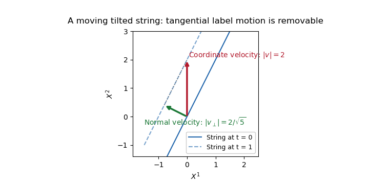
For the linear profile, the spatial string is the straight line $X^2=k{X}^1+kt$. It is tilted, and its coordinate intercept moves with speed $k$. This is also a uniformly moving straight string: the physical transverse velocity of a tilted string is the velocity normal to the line. With unit tangent $(1,k)/\sqrt{1+k^2}$ and coordinate velocity $(0,k)$, the normal speed isThus $k>1$ does not imply superluminal physical motion. Fixed-$\sigma$ labels have spacelike trajectories when $k>1$, but labels on a string can slide tangentially and are not identifiable material particles. Choosing $\dot{\sigma }=-k^2/(1+k^2)$ removes the tangential velocity and gives the subluminal velocity $(-k^2,k)/(1+k^2)$.

The induced worldsheet metric supplies a coordinate-invariant check:The string worldsheet remains Lorentzian for every finite $k$, including $k=1$ and $k>1$. Its constant energy density is $1+k^2$. This linear profile is a tilted boosted straight string, rather than a localized finite-energy wave.

In a point-particle description of quantum gravity, interactions of a massless spin-two field occur at localized vertices of Feynman diagrams. The gravitational coupling has negative mass dimension for spacetime dimension greater than two, so short-distance loop integrations generate higher-derivative counterterms that cannot all be absorbed into the Einstein action. A string worldsheet instead joins incoming and outgoing strings by a smooth surface. In particular, a closed string splits or joins through a smooth pair-of-pants surface. There is no invariantly distinguished point at which every part of an extended string interacts. The choice of a time slicing can draw a joining point, but it is not a physical pointlike vertex. This removes the point-interaction geometry responsible for arbitrarily localized interactions and introduces the string length ${\ell }_s=\sqrt{{\alpha }^{\prime }}$.

This geometric explanation is supported by the organization of the Polyakov path integral. Introducing a worldsheet metric makes the Nambu–Goto action amenable to gauge fixing. In the Euclidean integral, metrics on a fixed oriented surface are divided by worldsheet diffeomorphisms and Weyl transformations. What remains is a Riemann surface with a conformal structure, together with finitely many worldsheet moduli and the positions of external string vertex operators. The determinants from fixing the metric are represented by Faddeev-Popov ghosts. Schematically, for $n$ closed-string external states,Here ${\mathcal{M}}_{g,n}$ is the moduli space of genus-$g$ punctured surfaces. The dilaton weights a surface by its Euler characteristic $\chi =2-2g$, giving $g_s^{-\chi }$ before the normalization of external states. Every additional handle multiplies the contribution by $g_s^2$. The string genus expansion therefore plays the role of the ordinary loop expansion, with the sphere giving tree level and the torus giving one loop. The critical dimension cancels the worldsheet Weyl anomaly, making this reduction to conformal geometry consistent.

The massless symmetric traceless closed-string state is a graviton, and its long-wavelength interactions reproduce gravity. At distances comparable with ${\ell }_s$, however, an infinite tower of excited states contributes. This is more than a single particle form factor: the same amplitude contains graviton exchange, massive higher-spin exchange and string-scale softness.

The dimensionless variables in the given Virasoro–Shapiro amplitude correspond to $s={\alpha }^{\prime }S/4$, $t={\alpha }^{\prime }T/4$, $u={\alpha }^{\prime }U/4$, where capital letters denote the usual dimensionful Mandelstam invariants. Its constraint $s+t+u=-4$ identifies the external particles as the closed bosonic tachyons, not four gravitons. Nevertheless its intermediate massless pole directly exhibits graviton exchange. The overall normalization will be suppressed below; no additional copy of the amplitude formula is needed.

First, the amplitude is symmetric under permutations of $s,t,u$, expressing crossing symmetry. The poles in any channel areFor generic $t$, the residue can be calculated with the Gamma function pole at $-n$ and its recurrence:The product is $1$ when $n=0$. Indeed, the pole factor contributes $(-1{)}^{n+1}/n!$, while the two remaining Gamma ratios contribute $(-1{)}^n(t+2{)}_n^2/n!$. A residue polynomial of degree $2n$ shows exchange of spins up to $2n$, with leading Regge trajectory $J=2+2s$. At $n=1$, the massless residue is $-(t+2{)}^2$, containing the spin-two exchange. By crossing, the massless $t$-channel pole isfor generic $s$. Thus at large $s$ the pole behaves as $s^2/t$, the characteristic energy dependence of graviton exchange. Its massless propagator produces the long-range gravitational interaction. At low energies the massive poles can instead be expanded into local higher-derivative corrections to the effective gravitational action.

At the string scale one must retain the whole tower. The Gamma reflection formula rewrites the amplitude exactly asAt large $s$ and fixed $t$, away from the resonance poles or with a specified complex continuation, the Gamma ratio scales as $s^{t+1}$. Hence the Regge limit scales as $s^{2+2t}$, up to the signature factor and the displayed $t$-dependent coefficient. In particular, a fixed nonzero momentum transfer changes the point-graviton power law by a factor $s^{2t}$: the graviton belongs to an entire trajectory rather than remaining an isolated spin-two exchange at arbitrarily high energy.

There is stronger suppression when the scattering angle is fixed. Put $t\simeq -as$, $u\simeq -(1-a)s$ with $0<a<1$. Applying Stirling formula to the Gamma functions, after the same treatment of real-axis poles, gives the leading smooth envelopeThe leading $s\log s$ terms cancel and the remaining entropy-like combination is negative. In physical units the exponent is $-{\alpha }^{\prime }Sf(a)/2$. This fixed-angle softness of the closed-string amplitude is absent for an elementary pointlike gravitational vertex. Equivalently, short-distance gravitational scattering probes additional string degrees of freedom. In a four-dimensional long-distance effective setting, a massive exchanged mode contributes a Yukawa-type correction proportional to $e^{-M_{n}r}/r$, with couplings and tensor factors depending on the external states. Such terms are suppressed for $r\gg {\ell }_s$ and become relevant for $r\sim {\ell }_s$. The amplitude establishes the spectrum and short-distance change; it does not by itself give a universal static potential for arbitrary sources. Its bosonic tachyon also signals an unstable vacuum, so it must not be treated as a complete stable model of a gravitational force.

Finally, the modular group prevents overcounting equivalent surfaces and reorganizes the loop ultraviolet region. A torus is $\mathbb{C}/(\mathbb{Z}+\tau \mathbb{Z})$ with $\mathrm{Im}\tau >0$. A change of lattice basis identifiesThus the one-loop integral uses a fundamental domain for $\mathrm{PSL}(2,\mathbb{Z})$, for exampleThe measure $d^2\tau /(\mathrm{Im}\tau {)}^2$ is invariant, and the physical integrand, including matter, ghosts and external insertions, must respect torus modular invariance. In this domain $\mathrm{Im}\tau \ge \sqrt{3}/2$. The region of arbitrarily small proper time that causes ultraviolet divergences in a particle loop is therefore not an independent part of the string integral; a modular transformation relates it to another description already represented in the domain.

This does not remove every possible divergence. The cusp $\mathrm{Im}\tau \to \infty$ is a long tube, and factorization through it can produce infrared divergences, massless tadpoles or the bosonic tachyon divergence. At higher genus, degenerating cycles similarly factorize into propagating intermediate string states. The essential improvement is the relation between worldsheet geometry, the full spectrum and the quotient by large diffeomorphisms; infrared and unstable-background problems remain separate questions. A short-distance expansion that keeps only the graviton discards precisely this structure.

For each initial Kerr black hole, $r_{+}=M+\sqrt{M^2-a^2}$ and the horizon area follows by integrating its induced metric:The final Schwarzschild black hole has area $16\pi M^{\prime 2}$. Applying the second law of black-hole mechanics to the sum of the two initial areas givesConsequently the radiated energy fraction satisfiesThe bound is $1-1/\sqrt{2}\approx 0.293$ for nonrotating initial holes and tends to $1/2$ as $|a|/M\to 1$. It is an upper bound from area alone, not a predicted efficiency or an assurance that equality is realizable. A final Schwarzschild black hole has zero angular momentum; any nonzero total initial angular momentum must also be removed or compensated, which can further restrict a physical merger.

First construct the periodic response required in the introductory clause. At ${\omega }_0^2=1/(LC)$, the terms $L{I}_0^{\prime \prime }+I_0/C$ cancel for a sinusoid, leaving $R{I}_0^{\prime }={\omega }_0\cos ({\omega }_{0}t)$. ThusThis resonant series RLC response dissipates energy through Joule heating. Over one period,The Q factor, using the maximum magnetic energy $L{I}_M^2/2$, is consequently

Interpret projection from very far away as the asymptotic incoming state at $r\to \infty$. For $v>0$ and impact parameter $b>0$, conservation of energy and conservation of angular momentum give $E=v^2/2$ and $|h|=bv$. At the closest approach the radial velocity vanishes. With $k=-\kappa <0$, the central-force radial turning point equation isOnly the positive root is physical. Put $q=\kappa /v^2$. The pericentre distance and the purely tangential speed there areThus $p<b$ and $u>v$: attraction bends the path inward and increases the speed. With positive energy, the Kepler orbit is a hyperbola. Measured from the pericentre direction, its polar coordinates satisfy $r=h^2/[\kappa (1+e\cos \varphi )]$ with $e=\sqrt{1+b^2{v}^4/{\kappa }^2}>1$.

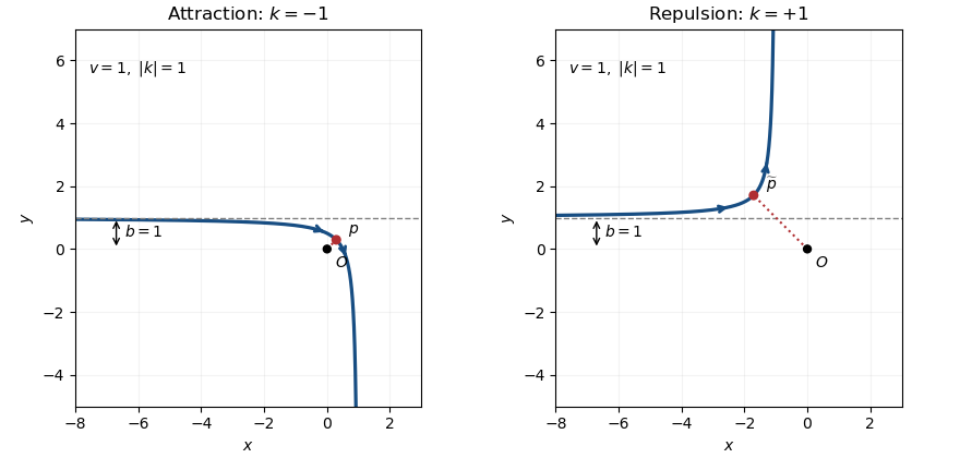
The hyperbola shown has a nonzero impact parameter. For $b=0$, the attractive radial orbit instead reaches the singular origin; there is no regular turning point with a finite closest-approach speed.

Use momentum conservation and conservation of energy in the laboratory inertial frame. The photon has momentum magnitude $E/c$, while the outgoing Electron satisfies the relativistic energy-momentum relation. Its total energy and momentum obeySubstitute these into $E_e^2=m^2{c}^4+c^2|{\mathbf{p}}_e{|}^2$. Cancelling $m^2{c}^4$ and $(E_1-E_2{)}^2$ gives $m{c}^2(E_1-E_2)=E_1{E}_2(1-\cos \theta )$. Both photon energies are positive, so division yieldsThis is Compton scattering. The energies include the Electron's rest energy; using only its kinetic energy in the mass-shell equation would give the wrong result. The outgoing photon has unchanged energy at $\theta =0$ and smaller energy for a nonzero scattering angle.

Let ${\mathbf{p}}_1$ and ${\mathbf{p}}_2$ be the incoming and proton momenta. The other incoming atom is at rest, so its total energy is $m_1{c}^2$. By four-momentum conservation, the tritium atom hasThe specified perpendicular emission gives ${\mathbf{p}}_1\cdot {\mathbf{p}}_2=0$. Therefore the relativistic energy-momentum relation impliesDividing by $c^4$ givesHere $E_1,E_2$ are total energies, not just kinetic energies. This identity is conditional on the collision admitting the stated emission: the calculated energies must satisfy the positive-energy mass-shell conditions, in particular $E_2\ge m_2{c}^2$ and $E_3\ge m_3{c}^2$. No nonrelativistic approximation has been used.

The wavefunction is a plane wave and a simultaneous formal eigenfunction of the momentum operator and the time-translation energy operator:Its momentum and energy are therefore definite, while its probability density is spatially uniform:For a particle of mass $m$, the probability current is $j=(\hslash /m)\mathrm{Im}(\overline{\varphi }{\partial }_x\varphi )=\hslash k{A}^2/m$, directed according to the sign of $k$.

On the whole real line, a nonzero constant-amplitude plane wave is not square-integrable and cannot be normalised to total probability one. It represents an idealised momentum eigenstate, interpreted through generalized eigenfunctions or as a limit of wave packets. Also, arbitrary $k,E$ do not automatically solve the Schrodinger equation for a specified potential energy: for a free particle, $E={\hslash }^2{k}^2/(2m)$, or this value plus the constant potential energy for a constant-potential region. If $A=0$, the zero function is not a physical quantum state.

Use a local first-derivative Lagrangian density $\mathcal{L}(\varphi ,{\partial }_{\mu }\varphi ,x)$ with sufficient differentiability, and let variations have compact support or vanish at the spacetime boundary. If the phrase “a function of the field” were read literally as forbidding derivatives, the equation below would reduce to $\partial \mathcal{L}/\partial \varphi =0$; a propagating field requires derivative dependence. Varying the action givesIntegration by parts and arbitrary interior variations yield the Euler-Lagrange field equation,The boundary condition is part of this derivation; if boundary variations are allowed, their separate boundary equations must also be imposed.

A variational symmetry of a Lagrangian density is an infinitesimal field change $\delta \varphi =\epsilon X$ for which $\delta \mathcal{L}=\epsilon {\partial }_{\mu }{K}^{\mu }$ off shell. Equality to zero is sufficient but is not necessary: a divergence changes only the boundary contribution to the action. For fixed-coordinate field variations,Equating the two expressions proves the scalar-field form of the Noether theorem:Thus every differentiable one-parameter variational symmetry gives a conserved current, and its Noether charge $Q=\int d^{3}x{j}^0$ is constant when the spatial boundary flux vanishes. This is the Noether current for a first-derivative scalar field; the same identity applies to several real components by summing over them. Identically conserved improvement terms can change its local expression without changing the charge under the same boundary assumptions.

For an active spacetime translation, ${\varphi }^{\prime }(x)=\varphi (x-a)$ and $\delta \varphi =-a^{\nu }{\partial }_{\nu }\varphi$. If the Lagrangian density has no explicit coordinate dependence, $\delta \mathcal{L}=-a^{\nu }{\partial }_{\nu }\mathcal{L}$, so $K^{\mu }=-a^{\mu }\mathcal{L}$. The Noether current is $j^{\mu }=-a^{\nu }{T}^{\mu }{}_{\nu }$, whereThese four translation currents are the canonical stress-energy tensor, also called the energy-momentum tensor. The sign in $j=-aT$ follows from the chosen active translation; the translation charges themselves can be labelled by $P_{\nu }=\int T^0{}_{\nu }{d}^{3}x$.

For the free real scalar field, take the standard kinetic term and mass term. Its Lagrangian density and Klein-Gordon equation areHere ${\Pi }^{\mu }={\partial }^{\mu }\varphi$, so $T^{\mu \nu }={\partial }^{\mu }\varphi {\partial }^{\nu }\varphi -{\eta }^{\mu \nu }\mathcal{L}$. Raising the charge index gives the four-momentum of a free real scalar field,The first is total energy, and the three components of the second are physical spatial momentum. With signature $(+,-,-,-)$, $P_i=-P^i$; this explains the opposite sign if the conserved quantities are instead written with lower spatial indices. For example, a plane wave proportional to $\cos (Et-\mathbf{k}\cdot \mathbf{x})$ has momentum density along $\mathbf{k}$, confirming the sign. All charges require convergence of the integrals and vanishing boundary flux, or periodic boundary conditions in a finite box.

For the complex scalar field, treat $\psi$ and ${\psi }^{\ast }$ as independent variables when varying, equivalently use their two real components. The global phase symmetry of a complex scalar field is $\psi \mapsto e^{-i\alpha }\psi$, ${\psi }^{\ast }\mapsto e^{i\alpha }{\psi }^{\ast }$ for constant $\alpha$. Both the kinetic term and $V(|\psi {|}^2)$ are invariant. This is a global internal symmetry of a classical field theory with circle group $U(1)$; a spacetime-dependent phase would require a gauge connection.

Choosing this orientation for the phase parameter gives the Noether charge of a complex scalar field:To check conservation directly, the Euler-Lagrange field equations are $\square \psi +V^{\prime }(|\psi {|}^2)\psi =0$ and their complex conjugates, assuming a real differentiable potential. Hence ${\partial }_{\mu }{j}^{\mu }=i({\psi }^{\ast }\square \psi -\psi \square {\psi }^{\ast })=0$. Reversing the phase-parameter orientation reverses the current and charge, which is merely a convention. For a scalar carrying electric charge $q$, the physical electric charge is $qQ$ after electromagnetic coupling. In a neutral theory the same global charge can instead label an internal conserved quantum number; the density alone does not identify it automatically with electricity.

With the mode normalization given, the oscillator canonical commutation relations are $[a_{\mathbf{p}},a_{\mathbf{q}}^{†}]=(2\pi {)}^3{\delta }^3(\mathbf{p}-\mathbf{q})$, with the other two commutators zero. Let $E_{\mathbf{p}}=\sqrt{{\mathbf{p}}^2+m^2}$ and $p^0=E_{\mathbf{p}}$. The convention compatible with the requested numerator iswithout an additional factor of $i$ outside the vacuum expectation value. Put $\tau =x^0-y^0$ and $\mathbf{r}=\mathbf{x}-\mathbf{y}$. The Fock vacuum is annihilated by $a_{\mathbf{p}}$, so only $a{a}^{†}$ contributes to the two Wightman functions. Consequently,In the second term we changed $\mathbf{p}\mapsto -\mathbf{p}$ to give the same spatial exponential.

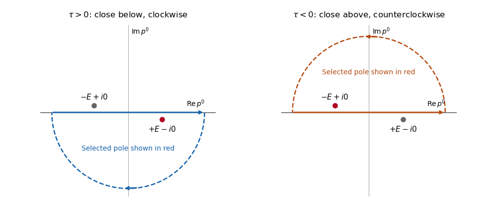
Now perform the energy contour integralHere the residue step uses $E>0$; the massless zero-momentum point is interpreted through the smeared distribution limit, not as an isolated normalized oscillator. The Feynman i-epsilon prescription puts the positive-energy pole below the real axis and the negative-energy pole above it: $p^0=E-i0$ and $p^0=-E+i0$. For $\tau >0$, close in the lower half-plane, clockwise; the residue theorem gives $-i$ times the residue $i{e}^{-iE\tau }/(2E)$, hence $e^{-iE\tau }/(2E)$. For $\tau <0$, close in the upper half-plane, counterclockwise; the negative-energy residue is $-i{e}^{iE\tau }/(2E)$, again giving a positive $e^{iE\tau }/(2E)$. These are exactly the two time-ordered terms. Restoring the spatial integral proves the scalar Feynman propagator pole prescription:The prescription in this formula supplies the pole convention left unspecified in the printed display; an unprescribed ordinary real-axis integral would not be well-defined. It is a distribution limit after smearing, not an absolutely convergent four-dimensional integral. With this normalization the derivative jump of a free scalar time-ordered two-point function gives $(\square +m^2){\Delta }_F=-i{\delta }^4(x-y)$, an independent check of both the numerator and the sign.

The pole displacement is exaggerated in this original schematic. The contour orientation and selected pole reproduce the time ordering of the Feynman propagator.

Use the real Lie-algebra convention of the question, with a gauge covariant derivative $D_{\mu }={\partial }_{\mu }+A_{\mu }$. The gauge field strength is its curvature:Write $a_{\mu }={\delta }_X{A}_{\mu }/ϵ=-{\partial }_{\mu }X+[X,A_{\mu }]$. To first order in $ϵ$,Substitute $a_{\mu }$. The mixed second derivatives of $X$ cancel. The terms containing first derivatives of $X$ cancel in pairs. The remaining terms areThe Jacobi identity combines the last two into $[X,[A_{\mu },A_{\nu }]]$. ConsequentlyThe transformation is homogeneous even though the connection transformation contains an inhomogeneous derivative term.

For a finite-dimensional Lie algebra, define its Adjoint representation by ${\mathrm{ad}}_X(Y)=[X,Y]$ and its Killing form byIt is a symmetric bilinear form by cyclicity of the trace. The Jacobi identity gives ${\mathrm{ad}}_{[Z,X]}=[{\mathrm{ad}}_Z,{\mathrm{ad}}_X]$. Set $A={\mathrm{ad}}_Z$, $B={\mathrm{ad}}_X$, $C={\mathrm{ad}}_Y$. ThenThis proves the invariant bilinear form on a Lie algebra property, without assuming simplicity or nondegeneracy.

For definiteness use the Minkowski metric $\eta =\mathrm{diag}(1,-1,-1,-1)$ and take a real compact semisimple Lie algebra as the gauge algebra. Its positive internal metric is $B=-\kappa$. A Killing-form Yang-Mills Lagrangian with the coupling absorbed into the connection isThe spacetime metric is unchanged by internal gauge transformations. HenceThus gauge invariance follows directly from invariance of the Killing form. Other overall conventions are possible, but the energy sign must be checked rather than inferred from a prefactor in isolation.

For physical kinetic terms the internal form must be real, nondegenerate and positive definite after choosing the overall sign. If ${\mathcal{E}}_i=F_{0i}$ and ${\mathcal{B}}_i=\frac{1}{2}{ϵ}_{ijk}{F}_{jk}$, the above convention has Lagrangian $[B({\mathcal{E}}_i,{\mathcal{E}}_i)-B({\mathcal{B}}_i,{\mathcal{B}}_i)]/(2g_{\mathrm{YM}}^2)$ and physical energy densityThe canonical Hamiltonian density also contains the nondynamical multiplier and a spatial divergence. With ${\Pi }_i={\mathcal{E}}_i/g_{\mathrm{YM}}^2$ and $D_i{\Pi }_i={\partial }_i{\Pi }_i+[A_i,{\Pi }_i]$, integration by parts using the invariant bilinear form on a Lie algebra givesThe Gauss law constraint in gauge theory sets $D_i{\Pi }_i=0$. If the boundary flux vanishes, or the appropriate boundary contribution is included, the integrated physical Hamiltonian is the positive energy displayed above.

An indefinite internal form would give gauge-field polarizations with opposite kinetic signs. A degenerate form would fail to supply a kinetic term for some directions. The compactness criterion from the Killing form says that negative-definiteness of the Killing form of a real finite-dimensional algebra is equivalent to compact semisimplicity; thus the pure Killing-form construction selects compact semisimple real forms. One cannot use a complex-bilinear Killing form on arbitrary complex field components as if it were a positive Hermitian metric.

This does not prohibit Abelian gauge theories. A compact Abelian factor has zero Killing form, so it needs a separately chosen positive invariant bilinear form on a Lie algebra, rather than the Killing form. More generally an algebra with a positive invariant metric on a Lie algebra is compact reductive, namely a direct sum of a compact semisimple algebra and an Abelian center. A noncompact group can also share the same compact Lie algebra through global covering choices in an Abelian factor; positivity is a statement about the algebra and internal metric, not by itself a classification of global gauge-group topology. Quantum matter anomalies and global restrictions would require additional input; no matter content is specified here.

For the finite matrix transformation, let $g(x)\in SU(N)$ and regard $g$ as a multiplication operator. The identity ${\partial }_{\mu }{g}^{-1}=-g^{-1}({\partial }_{\mu }g)g^{-1}$ givesTaking commutators of these differential operators cancels the adjacent multiplication operators $g^{-1}g$, yieldingThis argument keeps the derivatives acting on test fields and avoids treating $D_{\mu }$ as just a matrix.

There is a normalization issue in the printed last paragraph. The standard Killing form defined through the adjoint trace on $\mathfrak{su}(N)$ isnot simply $\mathrm{tr}(XY)$. For example, with $N=2$ and $X=Y=-i{\sigma }_3/2$, the defining trace is $-1/2$, whereas the adjoint trace is $-2$. The printed trace formula can be used as a rescaled invariant form, with the constant absorbed into the gauge coupling; it has exactly the invariance needed here. For either normalization,by cyclicity. This proves finite Yang-Mills gauge transformation invariance, with the healthy sign chosen for anti-Hermitian gauge fields. The normalization discrepancy is not a failure of gauge invariance.

Finally let $g(x)=e^{ϵX(x)}=I+ϵX(x)+O({ϵ}^2)$. Since $X\in \mathfrak{su}(N)$ is traceless and skew-Hermitian, this exponential lies in $SU(N)$. Expanding the finite formula givesThus the stated infinitesimal transformation is the derivative of the finite transformation at the identity. It describes transformations in the identity component; arbitrary global or large gauge transformations need not be generated by one globally defined infinitesimal parameter.